Chapter 15 An Introduction to Functional Programming
Functional Programming (FP) is another way of thinking about how to organize programs. We talked about OOP—another way to organize programs—in the last chapter (chapter 14). So how do OOP and FP differ? To put it simply, FP focuses on functions instead of objects. Because we are talking a lot about functions in this chapter, we will assume you have read and understood section 6.
Neither R nor Python is a purely functional language. For us, FP is a style that we can choose to let guide us, or that we can disregard. You can choose to employ a more functional style, or you can choose to use a more object-oriented style, or neither. Some people tend to prefer one style to other styles, and others prefer to decide which to use depending on the task at hand.
More specifically, a functional programming style takes advantage of first-class functions and favors functions that are pure.
- First-class functions are (Abelson and Sussman 1996) functions that
- can be passed as arguments to other functions,
- can be returned from other functions, and
- can be assigned to variables or stored in data structures.
- Pure functions
- return the same output if they are given the same input, and
- do not produce side-effects.
Side-effects are changes made to non-temporary variables, to the “state” of the program.
We discussed (1) in the beginning of chapter 6. If you have not used any other programming languages before, you might even take (1) for granted. However, using first-class functions can be difficult in other languages not mentioned in this text.
There is more to say about definition (2). This means you should keep your functions as modular as possible, unless you want your overall program to be much more difficult to understand. FP stipulates that
ideally functions will not refer to non-local variables;
ideally functions will not (refer to and) modify non-local variables; and
ideally functions will not modify their arguments.
Unfortunately, violating the first of these three criteria is very easy to do in both of our languages. Recall our conversation about dynamic lookup in subsection 6.8. Both R and Python use dynamic lookup, which means you can’t reliably control when functions look for variables. Typos in variable names easily go undiscovered, and modified global variables can potentially wreak havoc on your overall program.
Fortunately it is difficult to modify global variables inside functions in both R and Python. This was also discussed in subsection 6.8. In Python, you need to make use of the global keyword (mentioned in section 6.7.2), and in R, you need to use the rare super assignment operator (it looks like <<-, and it was mentioned in 6.7.1). Because these two symbols are so rare, they can serve as signals to viewers of your code about when and where (in which functions) global variables are being modified.
Last, violating the third criterion is easy in Python and difficult in R. This was discussed earlier in 6.7. Python can mutate/change arguments that have a mutable type because it has pass-by-assignment semantics (mentioned in section 6.7.2), and R generally can’t modify its arguments at all because it has pass-by-value semantics 6.7.1.
This chapter avoids the philosophical discussion of FP. Instead, it takes the applied approach, and provides instructions on how to use FP in your own programs. I try to give examples of how you can use FP, and when these tools are especially suitable.
One of the biggest tip-offs that you should be using functional programming is if you need to evaluate a single function many times, or in many different ways. This happens quite frequently in statistical computing. Instead of copy/pasting similar-looking lines of code, you might consider higher-order functions that take your function as an input, and intelligently call it in all the many ways you want it to. A third option you might also consider is to use a loop (c.f. 11.2). However, that approach is not very functional, and so it will not be heavily-discussed in this section.
Another tip-off that you need FP is if you need many different functions that are all “related” to one another. Should you define each function separately, using excessive copy/paste-ing? Or should you write a function that can elegantly generate any function you need?
Not repeating yourself and re-using code is a primary motivation, but it is not the only one. Another motivation for functional programming is clearly explained in Advanced R27:
A functional style tends to create functions that can easily be analysed in isolation (i.e. using only local information), and hence is often much easier to automatically optimise or parallelise.
All of these sound like a good things to have in our code, so let’s get started with some examples!
15.1 Functions as Function Inputs in R
Many of the most commonly-used functionals in R have names that end in “apply”. The ones I discuss are sapply(), vapply(), lapply(), apply(), tapply() and mapply(). Each of these takes a function as one of its arguments. Recall that this is made possible by the fact that R has first-class functions.
15.1.1 sapply() and vapply()
Suppose we have a data.frame that has 10 rows and 100 columns. What if we want to take the mean of each column?
An amateurish way to do this would be something like the following.
myFirstMean <- mean(myDF[,1])
mySecondMean <- mean(myDF[,2])
# ... so on and so forth ..
myHundredthMean <- mean(myDF[,100])
You will need one line of code for each column in the data frame! For data frames with a lot of columns, this becomes quite tedious. You should also ask yourself what happens to you and your collaborators when the data frame changes even slightly, or if you want to apply a different function to its columns. Third, the results are not stored in a single container. You are making it difficult on yourself if you want to use these variables in subsequent pieces of code.
“Don’t repeat yourself” (DRY) is an idea that’s been around for a while and is widely accepted (Hunt and Thomas 2000). DRY is the opposite of WET.
Instead, prefer the use of sapply() in this situation. The “s” in sapply() stands for “simplified.” In this bit of code mean() is called on each column of the data frame. sapply() applies the function over columns, instead of rows, because data frames are internally a list of columns.
myMeans <- sapply(myDF, mean)
myMeans[1:5]
##          X1          X2          X3          X4          X5
##  0.18577292  0.58759539 -0.05194271 -0.07027537 -0.35365358
Each call to mean() returns a double vector of length \(1\). This is necessary if you want to collect all the results into a vector–remember, all elements of a vector have to have the same type. To get the same behavior, you might also consider using vapply(myDF, mean, numeric(1)).
In the above case, “simplify” referred to how one-hundred length-\(1\) vectors were simplified into one length-\(100\) vector. However, “simplified” does not necessarily imply that all elements will be stored in a vector. Consider the summary function, which returns a double vector of length \(6\). In this case, one-hundred length-\(6\) vectors were simplified into one \(6 \times 100\) matrix.
mySummaries <- sapply(myDF, summary)
is.matrix(mySummaries)
## [1] TRUE
dim(mySummaries)
## [1]   6 100
Another function that is worth mentioning is replicate()–it is a wrapper for sapply(). Consider a situation where you want to call a function many times with the same inputs. You might try something like sapply(1:100, function(elem) { return(myFunc(someInput)) } ). Another, more readable, way to do this is replicate(100, myFunc(someInput)).
15.1.2 lapply()
For functions that do not return amenable types that fit into a vector, matrix or array, they might need to be stored in list. In this situation, you would need lapply(). The “l” in lapply() stands for “list”. lapply() always returns a list of the same length as the input.
regress <- function(y){ lm(y ~ 1) }
myRegs <- lapply(myDF, regress)
length(myRegs)
## [1] 100
class(myRegs[[1]])
## [1] "lm"
summary(myRegs[[12]])
##
## Call:
## lm(formula = y ~ 1)
##
## Residuals:
##     Min      1Q  Median      3Q     Max
## -1.6149 -0.8692 -0.2541  0.7596  2.5718
##
## Coefficients:
##             Estimate Std. Error t value Pr(>|t|)
## (Intercept)   0.2104     0.4139   0.508    0.623
##
## Residual standard error: 1.309 on 9 degrees of freedom
15.1.3 apply()
I use sapply() and lapply() the most, personally. The next most common function I use is apply(). You can use it to apply functions to rows of rectangular arrays instead of columns. However, it can also apply functions over columns, just as the other functions we discussed can.28
dim(myDF)
## [1]  10 100
results <- apply(myDF, 1, mean)
results[1:4]
## [1]  0.18971263 -0.07595286  0.18400138  0.08895979
Another example where it can be useful to apply a function to rows is predicate functions. A predicate function is just a fancy name for a function that returns a Boolean. I use them to filter out rows of a data.frame. Without a predicate function, filtering rows might look something like this on our real estate data (Albemarle County Geographic Data Services Office 2021) (Ford 2016).
albRealEstate <- read.csv("data/albemarle_real_estate.csv")
firstB <- albRealEstate$YearBuilt == 2006
secondB <- albRealEstate$Condition == "Average"
thirdB <- albRealEstate$City == "CROZET"
subDF <- albRealEstate[(firstB & secondB) | thirdB,]
str(subDF, strict.width = "cut")
## 'data.frame':    3865 obs. of  12 variables:
##  $ YearBuilt    : int  1769 1818 2004 2006 2004 1995 1900 1960 ..
##  $ YearRemodeled: int  1988 1991 NA NA NA NA NA NA NA NA ...
##  $ Condition    : chr  "Average" "Average" "Average" "Average" ..
##  $ NumStories   : num  1.7 2 1 1 1.5 2.3 2 1 1 1 ...
##  $ FinSqFt      : int  5216 5160 1512 2019 1950 2579 1530 800 9..
##  $ Bedroom      : int  4 6 3 3 3 3 4 2 2 2 ...
##  $ FullBath     : int  3 4 2 3 3 2 1 1 1 1 ...
##  $ HalfBath     : int  0 1 1 0 0 1 0 0 0 0 ...
##  $ TotalRooms   : int  8 11 9 10 8 8 6 4 4 4 ...
##  $ LotSize      : num  5.1 453.9 42.6 5 5.5 ...
##  $ TotalValue   : num  1096600 2978600 677800 453200 389200 ...
##  $ City         : chr  "CROZET" "CROZET" "CROZET" "CROZET" ...
Complicated filtering criteria can become quite wide, so I prefer to break the above code into three steps.
- Step 1: write a predicate function that returns TRUE or FALSE;
- Step 2: construct a
logicalvectorbyapply()ing the predicate over rows; - Step 3: plug the
logicalvectorinto the[operator to remove the rows.
pred <- function(row){
  yrBuiltCorrect <- row['YearBuilt'] == 2006
  aveCond <- row['Condition'] == "Average"
  inCrozet <- row['City'] == "CROZET"
  ( yrBuiltCorrect && aveCond) || inCrozet
}
whichRows <- apply(albRealEstate, 1, pred)
subDF <- albRealEstate[whichRows,]
str(subDF, strict.width = "cut")
## 'data.frame':    3865 obs. of  12 variables:
##  $ YearBuilt    : int  1769 1818 2004 2006 2004 1995 1900 1960 ..
##  $ YearRemodeled: int  1988 1991 NA NA NA NA NA NA NA NA ...
##  $ Condition    : chr  "Average" "Average" "Average" "Average" ..
##  $ NumStories   : num  1.7 2 1 1 1.5 2.3 2 1 1 1 ...
##  $ FinSqFt      : int  5216 5160 1512 2019 1950 2579 1530 800 9..
##  $ Bedroom      : int  4 6 3 3 3 3 4 2 2 2 ...
##  $ FullBath     : int  3 4 2 3 3 2 1 1 1 1 ...
##  $ HalfBath     : int  0 1 1 0 0 1 0 0 0 0 ...
##  $ TotalRooms   : int  8 11 9 10 8 8 6 4 4 4 ...
##  $ LotSize      : num  5.1 453.9 42.6 5 5.5 ...
##  $ TotalValue   : num  1096600 2978600 677800 453200 389200 ...
##  $ City         : chr  "CROZET" "CROZET" "CROZET" "CROZET" ...
15.1.4 tapply()
tapply() can be very handy when you need it. First, we’ve alluded to the definition before in subsection 8.1, but a ragged array is a collection of arrays that all have potentially different lengths. I don’t typically construct such an object and then pass it to tapply(). Rather, I let tapply() construct the ragged array for me. The first argument it expects is, to quote the documentation, “typically vector-like,” while the second tells us how to break that vector into chunks. The third argument is a function that gets applied to each vector chunk.
If I wanted the average home price for each city, I could use something like this.
str(albRealEstate, strict.width = "cut")
## 'data.frame':    30381 obs. of  12 variables:
##  $ YearBuilt    : int  1769 1818 2004 2006 2004 1995 1900 1960 ..
##  $ YearRemodeled: int  1988 1991 NA NA NA NA NA NA NA NA ...
##  $ Condition    : chr  "Average" "Average" "Average" "Average" ..
##  $ NumStories   : num  1.7 2 1 1 1.5 2.3 2 1 1 1 ...
##  $ FinSqFt      : int  5216 5160 1512 2019 1950 2579 1530 800 9..
##  $ Bedroom      : int  4 6 3 3 3 3 4 2 2 2 ...
##  $ FullBath     : int  3 4 2 3 3 2 1 1 1 1 ...
##  $ HalfBath     : int  0 1 1 0 0 1 0 0 0 0 ...
##  $ TotalRooms   : int  8 11 9 10 8 8 6 4 4 4 ...
##  $ LotSize      : num  5.1 453.9 42.6 5 5.5 ...
##  $ TotalValue   : num  1096600 2978600 677800 453200 389200 ...
##  $ City         : chr  "CROZET" "CROZET" "CROZET" "CROZET" ...
length(unique(albRealEstate$City))
## [1] 6
tapply(albRealEstate$TotalValue, list(albRealEstate$City), mean)[1:4]
## CHARLOTTESVILLE          CROZET     EARLYSVILLE         KESWICK
##        429926.5        436090.5        482711.4        565985.1
You might be wondering why we put albRealEstate$City into a list. That seems kind of unnecessary. This is because tapply() can be used with multiple factors–this will break down the vector input into a finer partition. The second argument must be one object, though, so all of these factors must be collected into a list. The following code produces a “pivot table.”
pivTable <- tapply(albRealEstate$TotalValue,
                   list(albRealEstate$City, albRealEstate$Condition),
                   mean)
pivTable[,1:5]
##                  Average Excellent     Fair     Good     Poor
## CHARLOTTESVILLE 416769.9  625887.9 306380.7 529573.4 304922.4
## CROZET          447585.8  401553.5 241568.8 466798.5 224516.2
## EARLYSVILLE     491269.6  492848.4 286980.0 522938.5 250773.3
## KESWICK         565994.3  664443.5 274270.4 676312.6 172425.0
## NORTH GARDEN    413788.8  529108.3 164646.2 591502.8 161460.0
## SCOTTSVILLE     286787.4  534500.0 196003.4 415207.5 183942.3
For functions that return higher-dimensional output, you will have to use something like by() or aggregate() in place of tapply().
15.1.5 mapply()
The documentation of mapply() states mapply() is a multivariate version of sapply(). sapply() worked with univariate functions; the function was called multiple times, but each time with a single argument. If you have a function that takes multiple arguments, and you want those arguments to change each time the function is called, then you might be able to use mapply().
Here is a short example. Regarding the n= argument of rnorm(), the documentation explains, “[i]f length(n) > 1, the length is taken to be the number required.” This would be a problem if we want to sample three times from a mean \(0\) normal first, then twice from a mean \(100\) normal, and then third, once from a mean \(42\) normal distribution. We only get three samples when we want six!
## [1] 0.01435773 99.99238144 42.01743548## [[1]]
## [1] -0.0122999207 -0.0064744814 -0.0002297629
##
## [[2]]
## [1] 100.02077 99.99853
##
## [[3]]
## [1] 41.9970415.1.6 Reduce() and do.call()
Unlike the other examples of functions that take other functions as inputs, Reduce() and do.call() don’t have many outputs. Instead of collecting many outputs into a container, they just output one thing.
Let’s start with an example: “combining” data sets. In section 12 we talked about several different ways of combining data sets. We discussed stacking data sets on top of one another with rbind() (c.f. subsection 12.2), stacking them side-by-side with cbind() (also in 12.2), and intelligently joining them together with merge() (c.f. 12.3).
Now consider the task of combining many data sets. How can we combine three or more data sets into one? Also, how do we write DRY code and abide by the DRY principle? As the name of the subsection suggests, we can use either Reduce() or do.call() as a higher-order function. Just like the aforementioned *apply() functions, they take in either cbind(), rbind(), or merge() as a function input. Which one do we pick, though? The answer to that question deals with how many arguments our lower-order function takes.
Take a look at the documentation to rbind(). Its first argument is ..., which is the dot-dot-dot symbol. This means rbind() can take a varying number of data.frames to stack on top of each other. In other words, rbind() is variadic.
On the other hand, take a look at the documentation of merge(). It only takes two data.frames at a time29. If we want to combine many data sets, merge() needs a helper function.
This is the difference between Reduce() and do.call(). do.call() calls a function once on many arguments, so its function must be able to handle many arguments. On the other hand, Reduce() calls a binary function many times on pairs of arguments. Reduce()’s function argument gets called on the first two elements, then on the first output and the third element, then on the second output and fourth element, and so on.
Here is an initial example that makes use of four data sets d1.csv, d2.csv, d3.csv, and d4.csv. To start, ask yourself how we would read all of these in. There is a temptation to copy and paste read.csv calls, but that would violate the DRY principle. Instead, let’s use lapply() an anonymous function that constructs a file path string, and then uses it to read in the data set the string refers to.
numDataSets <- 4
dataSets <- paste0("d",1:numDataSets)
dfs <- lapply(dataSets,
              function(name) read.csv(paste0("data/", name, ".csv")))
head(dfs[[3]])
##   id obs3
## 1  a    7
## 2  b    8
## 3  c    9
Notice how the above code would only need to be changed by one character if we wanted to increase the number of data sets being read in!30
Next, cbind()ing them all together can be done as follows. do.call() will call the function only once. cbind() takes many arguments at once, so this works. This code is even better than the above code in that if dfs becomes longer, or changes at all, nothing will need to be changed.
do.call(cbind, dfs) # DRY! :)
##   id obs1 id obs2 id obs3 id obs4
## 1  a    1  b    5  a    7  a   10
## 2  b    2  a    4  b    8  b   11
## 3  c    3  c    6  c    9  c   12
# cbind(df1,df2,df3,df4) # WET! :(
What if we wanted to merge() all these data sets together? After all, the id column appears to be repeating itself, and some data from d2 isn’t lining up.
Again, this is very DRY code. Nothing would need to be changed if dfs grew. Furthermore, trying to do.call() the merge() function wouldn’t work because it can only take two data sets at a time.
15.2 Functions as Function Inputs in Python
15.2.1 Functions as Function Inputs in Base Python
I discuss two functions from base Python that take functions as input. Neither return a list or a np.array, but they do return different kinds of iterables, which are “objects capable of returning their members one at a time,” according to the Python documentation. map(), the function, will return objects of type map. filter(), the function, will return objects of type filter. Often times we will just convert these to the container we are more familiar with.
15.2.1.1 map()
map() can call a function repeatedly using elements of a container as inputs. Here is an example of calculating outputs of a spline function, which can be useful for coming up with predictors in regression models. This particular spline function is \(f(x) = (x-k)1(x \ge k)\), where \(k\) is some chosen “knot point.”
import numpy as np
my_inputs = np.linspace(start = 0, stop = 2*np.pi)
def spline(x):
    knot = 3.0
    if x >= knot:
        return x-knot
    else:
        return 0.0
output = list(map(spline, my_inputs))
We can visualize the mathematical function by plotting its outputs against its inputs. More information on visualization was given in subsection 13.
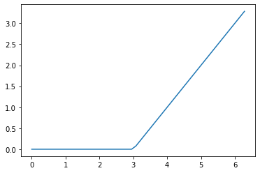
Figure 15.1: Our Spline Function
map() can also be used like mapply(). In other words, you can apply it to two containers,
15.2.1.2 filter()
filter() helps remove unwanted elements from a container. It returns an iterable of type filter, which we can iterate over or convert to a more familiar type of container. In this example, I iterate over it without converting it.
This code also provides our first example of a lambda function (Lutz 2013). Lambda functions are simply another way to define functions. Notice that in this example, we didn’t have to name our function. In other words, it was anonymous. We can also save a few lines of code.
15.2.2 Functions as Function Inputs in Numpy
Numpy provides a number of functions that facilitate working with np.ndarrays in a functional style. For example, np.apply_along_axis() is similar to R’s apply(). apply() had a MARGIN= input (1 sums rows, 2 sums columns), whereas this function has a axis= input (0 sums columns, 1 sums rows).
15.2.3 Functional Methods in Pandas
Pandas’ DataFrames have an .apply() method that is very similar to apply() in R,31 but again, just like the above function, you have to think about an axis= argument instead of a MARGIN= argument.
import pandas as pd
alb_real_est = pd.read_csv("data/albemarle_real_estate.csv")
alb_real_est.shape
## (30381, 12)
alb_real_est.apply(len, axis=0) # length of columns
## YearBuilt        30381
## YearRemodeled    30381
## Condition        30381
## NumStories       30381
## FinSqFt          30381
## Bedroom          30381
## FullBath         30381
## HalfBath         30381
## TotalRooms       30381
## LotSize          30381
## TotalValue       30381
## City             30381
## dtype: int64
type(alb_real_est.apply(len, axis=1)) # length of rows
## <class 'pandas.core.series.Series'>
Another thing to keep in mind is that DataFrames, unlike ndarrays, don’t have to have the same type for all elements. If you have mixed column types, then summing rows, for instance, might not make sense. This just requires subsetting columns before .apply()ing a function to rows. Here is an example of computing each property’s “score”.
import pandas as pd
# alb_real_est.apply(sum, axis=1) # can't add letters to numbers!
def get_prop_score(row):
    return 2*row[0] + 3*row[1]
two_col_df = alb_real_est[['FinSqFt','LotSize']]
alb_real_est['Score'] = two_col_df.apply(get_prop_score, 1)
alb_real_est[['FinSqFt','LotSize','Score']].head(2)
##    FinSqFt  LotSize      Score
## 0     5216    5.102  10447.306
## 1     5160  453.893  11681.679
.apply() also works with more than one function at a time.
alb_real_est[['FinSqFt','LotSize']].apply([sum, len])
##       FinSqFt      LotSize
## sum  61730306  105063.1892
## len     30381   30381.0000
If you do not want to waste two lines defining a function with def, you can use an anonymous lambda function. Be careful, though–if your function is complex enough, then your lines will get quite wide. For instance, this example is pushing it.
two_col_df.apply(lambda row : sum(row*[2,3]), 1)[:3]
## 0    10447.306
## 1    11681.679
## 2     3151.770
## dtype: float64
The previous example .apply()s a binary function to each row. The function is binary because it takes two elements at a time. If you want to apply a unary function (i.e. it takes one argument at a time) function to each row for, and for each column, then you can use .applymap().
alb_real_est[['FinSqFt','LotSize']].applymap(lambda e : e + 1).head(3)
##    FinSqFt  LotSize
## 0     5217    6.102
## 1     5161  454.893
## 2     1513   43.590
Last, we have a .groupby() method, which can be used to mirror the behavior of R’s tapply(), aggregate() or by(). It can take the DataFrame it belongs to, and group its rows into multiple sub-DataFrames. The collection of sub-DataFrames has a lot of the same methods that an individual DataFrame has (e.g. the subsetting operators, and the .apply() method), which can all be used in a second step of calculating things on each sub-DataFrame.
type(alb_real_est.groupby(['City']))
## pandas.core.groupby.generic.DataFrameGroupBy
type(alb_real_est.groupby(['City'])['TotalValue'])
## pandas.core.groupby.generic.SeriesGroupBy
Here is an example that models some pretty typical functionality. It shows two ways to get the average home price by city. The first line groups the rows by which City they are in, extracts the TotalValue column in each sub-DataFrame, and then .apply()s the np.average() function on the sole column found in each sub-DataFrame. The second .apply()s a lambda function to each sub-DataFrame directly. More details on this “split-apply-combine” strategy can be found in the Pandas documentation.
grouped = alb_real_est.groupby(['City'])
grouped['TotalValue'].apply(np.average)
## City
## CHARLOTTESVILLE    429926.502708
## CROZET             436090.502541
## EARLYSVILLE        482711.437566
## KESWICK            565985.092025
## NORTH GARDEN       399430.221519
## SCOTTSVILLE        293666.758242
## Name: TotalValue, dtype: float64
grouped.apply(lambda df : np.average(df['TotalValue']))
## City
## CHARLOTTESVILLE    429926.502708
## CROZET             436090.502541
## EARLYSVILLE        482711.437566
## KESWICK            565985.092025
## NORTH GARDEN       399430.221519
## SCOTTSVILLE        293666.758242
## dtype: float64
15.3 Functions as Function Outputs in R
Functions that create and return other functions are sometimes called function factories. Functions are first-class objects in R, so it’s easy to return them. What’s more interesting is that supposedly temporary objects inside the outer function can be accessed during the call of the inner function after it’s returned.
Here is a first quick example.
funcFactory <- function(greetingMessage){
  function(name){
    paste(greetingMessage, name)
  }
}
greetWithHello <- funcFactory("Hello")
greetWithHello("Taylor")
## [1] "Hello Taylor"
greetWithHello("Charlie")
## [1] "Hello Charlie"
Notice that the greetingMessage= argument that is passed in, "Hello", isn’t temporary anymore. It lives on so it can be used by all the functions created by funcFactory(). This is the most surprising aspect of writing function factories.
Let’s now consider a more complicated and realistic example. Let’s implement a variance reduction technique called common random numbers.
Suppose \(X \sim \text{Normal}(\mu, \sigma^2)\), and we are interested in approximating an expectation of a function of this random variable. Suppose that we don’t know that
\[\begin{equation}
\mathbb{E}[\sin(X)] = \sin(\mu) \exp\left(-\frac{\sigma^2}{2}\right)
\end{equation}\]
for any particular choice of \(\mu\) and \(\sigma^2\), and instead, we choose to use the Monte Carlo method:
\[\begin{equation}
\hat{\mathbb{E}}[\sin(X)] = \frac{1}{n}\sum_{i=1}^n\sin(X^i)
\end{equation}\]
where \(X^1, \ldots, X^n \overset{\text{iid}}{\sim} \text{Normal}(\mu, \sigma^2)\) is a large collection of draws from the appropriate normal distribution, probably coming from a call to rnorm(). In more realistic situations, the theoretical expectation might not be tractable, either because the random variable has a complicated distribution, or maybe because the functional is very complicated. In these cases, a tool like Monte Carlo might be the only available approach.
Here are two functions that calculate the above quantities for \(n=1000\). actualExpectSin() is a function that computes the theoretical expectation for any particular parameter pair. monteCarloSin() is a function that implements the Monte Carlo approximate expectation.
n <- 1000 # don't hardcode variables that aren't passed as arguments!
actualExpectSin <- function(params){
  stopifnot(params[2] > 0) # second parameter is sigma
  sin(params[1])*exp(-.5*(params[2]^2))
}
monteCarloSin <- function(params){
  stopifnot(params[2] > 0)
  mean(sin(rnorm(n = n, mean = params[1], sd = params[2])))
}
# monteCarloSin(c(10,1))
One-off approximations aren’t as interesting as visualizing many expectations for many parameter inputs. Below we plot the expectations for many different parameter vectors/configurations/settings.
muGrid <- seq(-10,10, length.out = 100)
sigmaGrid <- seq(.001, 5, length.out = 100)
muSigmaGrid <- expand.grid(muGrid, sigmaGrid)
actuals <-  matrix(apply(muSigmaGrid, 1, actualExpectSin),
                   ncol = length(muGrid))
mcApprox <- matrix(apply(muSigmaGrid, 1, monteCarloSin),
                   ncol = length(muGrid))

par(mfrow=c(1,2))
contour(muGrid, sigmaGrid, actuals,
        xlab = "mu", ylab = "sigma", main = "actual expects")
contour(muGrid, sigmaGrid, mcApprox,
        xlab = "mu", ylab = "sigma", main = "mc without crn")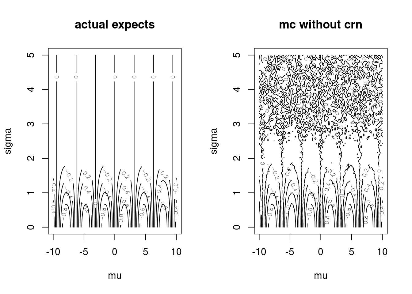
Figure 15.2: Monte Carlo Approximations versus Exact Evaluations
There are three problems with this implementation:
monteCarloSin()is not pure because it captures thenvariable,- the only way to increase the accuracy of the plot in the right panel is to increase
n, and - every time we re-run this code the plot on the right looks different.
If we wanted to use common random numbers, we could generate \(Z^1, \ldots, Z^n \overset{\text{iid}}{\sim} \text{Normal}(0, 1)\), and use the fact that
\[\begin{equation} X^i = \mu + \sigma Z^i \end{equation}\]
This leads to the Monte Carlo estimate
\[\begin{equation} \tilde{\mathbb{E}}[\sin(X)] = \frac{1}{n}\sum_{i=1}^n\sin(\mu + \sigma Z^i) \end{equation}\]
Here is one function that naively implements Monte Carlo with common random numbers. We generate the collection of standard normal random variables once, globally. Each time you call monteCarloSinCRNv1(c(10,1)), you get the same answer.
commonZs <- rnorm(n=n)
monteCarloSinCRNv1 <- function(params){
  stopifnot(params[2] > 0)
  mean(sin(params[1] + params[2]*commonZs))
}
# monteCarloSinCRNv1(c(10,1))
Let’s compare using common random numbers to going without. As you can see, common random numbers make the plot look “smoother.” In other words, we increase our sampling accuracy without spending more computational time.
mcApproxCRNv1 <- matrix(apply(muSigmaGrid, 1, monteCarloSinCRNv1),
                        ncol = length(muGrid))
par(mfrow=c(1,2))
contour(muGrid, sigmaGrid, mcApprox,
        xlab = "mu", ylab = "sigma", main = "mc without crn")
contour(muGrid, sigmaGrid, mcApproxCRNv1,
        xlab = "mu", ylab = "sigma", main = "mc with crn")
Figure 15.3: Monte Carlo: With and Without Common Random Numbers
There are some new downsides to this implementation to consider:
- we have another global variable–a bunch of samples called
commonZsfloating around, and - the dependence on the global variable for sample size is even further obscured.
We can fix these two problems very nicely by using a function factory.
makeMCFunc <- function(n = 1000){
  commonZs <- rnorm(n)
  function(params){
    stopifnot(params[2] > 0)
    mean(sin(params[1] + params[2]*commonZs))
  }
}
monteCarloSinCRNv2 <- makeMCFunc()
# now call monteCarloSinCRNv2 to approx. expectations
# e.g. monteCarloSinCRNv2(c(10,1))
This is much better because
- the desired sample size must be passed in as a function argument instead of being captured,
- the re-used standard normal variates are not in the global environment anymore, and
- a sensible default number of samples is provided in the event that the programmer forgets to specify one.
The inner function did in fact capture commonZs, but it captured from the enclosing scope, not the global scope. Capturing isn’t always a terrible idea. It would be difficult to modify these variables, so we don’t need to worry about function behavior changing in unpredictable ways. Actually capturing a variable instead of passing it in is an intelligent design choice–now the end-users of functions created by this factory don’t need to worry about plugging in extra parameters.
Let’s use \(1000\) samples again and make sure this function works by comparing its output to the known true function. Run the following code on your own machine. Note the new Greek letters in the axis labels.
mcApproxCRNv2 <- matrix(apply(muSigmaGrid, 1, monteCarloSinCRNv2),
                        ncol = length(muGrid))
par(mfrow=c(1,2))
contour(muGrid, sigmaGrid, mcApprox,
        xlab = expression(mu), ylab = expression(sigma))
contour(muGrid, sigmaGrid, mcApproxCRNv2,
        xlab = expression(mu), ylab = expression(sigma))
par(mfrow=c(1,1))
15.4 Functions as Function Outputs in Python
We can write function factories in Python, too. Here is another implementation of the first example from the previous section. Again, just as it did in R, str passed in as greeting_message persists well after func_factory() is finished working.
def func_factory(greeting_message):
    def func(name):
        print(greeting_message + ' ' + name)
    return func
greet_with_hello = func_factory("Hello")
greet_with_hello("Taylor")
## Hello Taylor
greet_with_hello("Charlie")
## Hello Charlie
Let’s consider another less trivial example. Recall the spline function from earlier in the chapter:
This function is limited in that it takes in only one element at a time. Unfortunately, we would not be able to provide an entire Numpy array as an argument (e.g. spline(np.arange(3))). Many functions do possess this behavior, and it is generally advantageous to take advantage of it. If you recall our discussion about universal functions in section 3.4, you might have grown accustomed to taking advantage of writing vectorized code.
Fortunately there’s a way to automatically vectorize functions like the one above: np.vectorize(). np.vectorize() takes in a unary function, and outputs a vectorized version of it that is able to take entire arrays as an input. Here’s an example. Compare this to us using map() before.
my_inputs = np.linspace(start = 0, stop = 2*np.pi)
# make a vectorized function
vec_spline = np.vectorize(spline)
vec_spline(my_inputs)[:4]
# alternatively output = list(map(spline, my_inputs)) from last time
## array([0., 0., 0., 0.])
The above code doesn’t just demonstrate how to return functions from a function. It is also an example of using functions as function inputs. When a function takes in and spits out functions, there is an alternative way to use it that is unique to Python. You can use function decorators. You can decorate a function by using the @ operator (Lutz 2013).
If you decorate a function, it is equivalent to passing that function in to a function factory (aka outer function). That function will take the function you defined, alter it, and then give it back to you with the same name that you chose in the first place.
# instead of spline = np.vectorize(spline)
@np.vectorize
def spline(x):
    knot = 3.0
    if x >= knot:
        return x-knot
    else:
        return 0.0
spline(my_inputs)[:4]
## array([0., 0., 0., 0.])
15.4.1 Writing Our Own Decorators
We can write our own function factory that can be used as decoration. The main restriction is that this function factory must take a function as an argument, too. This can sometimes be restrictive. You might have noticed that the definition of func_factory() from earlier in this section did not do that. If you don’t believe me, as an exercise, after you read this section, you might consider trying to rewrite the example from 15.3 that implements Monte Carlo sampling using common random numbers.
Before we get too ahead of ourselves, let’s describe the basics. Here is our first decorator function add_greeting().
The decorator add_greeting() returns a function that is an embellished version of the function it is given. When we decorate a function with it, it looks like this.
You could get the same behavior by typing the following. They are equivalent!
Things can get a little more complicated when your decorators take additional arguments.
@add_greeting("How you doin'")
def print_name(first_name):
    print(first_name)
print_name('Taylor')
## How you doin'
## Taylor
So how do we write decorators that accomplish this? The important thing to remember is that @add_greeting("How you doin'") in the previous code block is equivalent to writing this after the function definition: print_name = add_greeting("How you doin'")(print_name). This is a function returning a function returning a function! The definition of add_greeting() could look something like this.
def add_greeting(greet):
    def decorator(func):
        def wrapper(name):
            print(greet)
            func(name)
        return wrapper
    return decorator
Now that you know how decorators work, you can feel comfortable using third-party ones. You might come across, for example, the @jit decorator from Numba, which will translate your Python function into faster machine code, the @lru_cache decorator from the functools module–this can make your code faster by saving some of its outputs–or decorators that perform application specific tasks like @tf.function from Tensorflow.
15.5 Exercises
15.5.1 Python Questions
Write a function decorator called @log_dens_eval(left_bound, right_bound). When it decorates a function, say func(x), it will not change that function’s input or output, but it will verify that the input to the function (in this case x) is between left_bound and right_bound. If it is not, it will return negative infinity.
The Split-Apply-Combine strategy might be useful in writing code for a tree-based model (Breiman et al. 1984). We won’t discuss how these models are estimated, but we will write a function that generates another function that is able to generate predictions by stratifying the input/predictor/feature space.
- Import the data
"winequality-red.csv", call itwine, and remove all columns except forfixed acidity,volatile acidity, andquality. - Write a function called
generate_pred_func(fixed_cutoff, vol_cutoff, dataset).- The
datasetargument should be a PandasDataFramethat has three columns calledfixed acidity,volatile acidity, andquality. - The
fixed_cutoffargument should be a floating point number that separatesfixed acidityinto two regions. - The
vol_cutoffargument should be a floating point number that separatesvolatile acidityinto two regions. - The function should return a function, say
func(fixed_acidity, volatile_acidity). The two arguments are floating points. This function should return the most frequentqualityobservation out of all points whose inputs lie in in the corresponding region in the feature space.
- The
After you finish the problem, you should have a definition of a generate_pred_func() that could be used as follows:
Let’s predict what type of activity some is doing based on measurements taken from their cell phone. We will begin implementing a K-Nearest Neighbors (KNN) classifier (Fix and Hodges 1989) (Cover and Hart 1967).
Consider the data files "X_train.txt" and "y_train.txt" from (Anguita et al. 2013), which is available from the UCI Machine Learning Repository (Dua and Graff 2017). The first data set consists of recorded movements from a cell phone, and the second data set consists of activity labels of people. Labels \(1\) through \(6\) correspond to walking, walking upstairs, walking downstairs, sitting, standing and laying, respectively.
- Read in
"X_train.txt"as aDataFramecalledx_train. - Read in
"y_train.txt"as aDataFramecalledy_train - Define a function called
standardize(arr)that takes in an array-like and returns a standardized version of the array-like. Do this by subtracting from each element the overall mean and dividing each element by the standard deviation (use the length as a denominator, not length minus \(1\)). - Apply
standardize()to each column and transformx_trainby replacing all of its column by their standardized versions. Make sure to overwritex_train. Do this in one line of code. - Write a function called
euclid_dist(arr1, arr2)that calculates Euclidean distance between two points/array-likes. - What is the most common label among the 5 rows that are closest to the first row? Assign your answer to
my_predict. Assume that the two data sets you imported have the same order. Don’t include the first row in these \(5\) nearest neighbors. Take care not to modifyx_trainory_train.
15.5.2 R Questions
The density of a particular bivariate Gaussian distribution is
\[ f(x,y) = \frac{1}{2 \pi} \exp\left[ -\frac{x ^2 + y^2}{2} \right] \tag{1}. \] The random elements \(X\) and \(Y\), in this particular case, are independent, each have unit variance, and zero mean. In this case, the marginal for \(X\) is a mean \(0\), unit variance normal distribution:
\[ g(x) = \frac{1}{\sqrt{2\pi}} \exp\left[ -\frac{x ^2 }{2} \right] \tag{2}. \]
- Write a function called
fTwoArgs(x,y)that takes two arguments, and returns the value of the above density in equation (1) at those two points. - Write a function called
fOneArg(vec)that takes one argument: a length twovector. It should return a density in equation (1) evaluated at that point. - Write a function called
gOneArg(x)that evaluates the density in (2). - Generate two sequences called
xPointsandyPoints. Have them contain the twenty equally-spaced numbers going from \(-3\) to \(3\), inclusive. - Use
expand.grid()to create adata.framecalledmyGrid. It should have two columns, and it should contain in its rows every possible pair of two points from the above sequences. The “x” coordinates should be in the first column. - Use
mapply()to evaluate the bivariate density on every grid point. Store your results in avectormEvals. - Use
apply()to evaluate the bivariate density on every grid point. Store your results in avectoraEvals. - Use
sapply()to evaluate the univariate density on every element ofxPoints. Store your results in avectorsEvals. - Use
vapplyto evaluate the univariate density on every element ofxPoints. Store your results invectorvEvals. - Use
lapplyto evaluate the univariate density on every element ofxPoints. Store your results in alistlEvals. - Generate two plots of the bivariate density. For one, use
persp(). For the other, usecontour(). Feel free to revive the code you used in Chapter 13’s Exercise 1. - Generate a third plot of the univariate density. Feel free to revive the code you used in Chapter 13’s Exercises.
Write a function that reads in all of the data sets contained in any given folder.
- The function should be called
readAllData(path, extensions). - The first argument,
path, should be a string representing which folder you would like to search for files. - The second argument,
extensions, should be acharactervectorof all the file extensions you are interested in reading in (e.g.c('.txt','.csv')). Be careful about using regular expressions! - The function should return a
listofdata.frames.
Consider the Militarized Interstate Disputes (v5.0) (Palmer et al.) data sets again: "MIDA 5.0.csv", "MIDB 5.0.csv", "MIDI 5.0.csv", and "MIDIP 5.0.csv".
- Read these data sets in as a
listofdata.frames. Call itdfList. - Use
lapply()anddo.call()to calculate the biggest column average for all of these data sets. Store this average asbiggestAve. Store the name of the column that had this biggest average aswhichBiggestAve. Don’t worry about storing which data set this column mean was found in. - Use
Reduce()andlapply()to, once again, calculate the biggest column average. Store this number asbiggestAve2
Abelson, Harold, and Gerald J. Sussman. 1996. Structure and Interpretation of Computer Programs. 2nd ed. Cambridge, MA, USA: MIT Press.
“Adult.” 1996. UCI Machine Learning Repository.
Albemarle County Geographic Data Services Office. 2021. “Albemarle County GIS Web.” https://www.albemarle.org/government/community-development/gis-mapping/gis-data.
Albon, Chris. 2018. Machine Learning with Python Cookbook: Practical Solutions from Preprocessing to Deep Learning. 1st ed. O’Reilly Media, Inc.
Anguita, D., Alessandro Ghio, L. Oneto, Xavier Parra, and Jorge Luis Reyes-Ortiz. 2013. “A Public Domain Dataset for Human Activity Recognition Using Smartphones.” In ESANN.
Beazley, David M., and Brian K. (Brian Kenneth) Jones. 2014. Python Cookbook: Recipes for Mastering Python 3. Third. pub-ora-media:adr: pub-ora-media.
Breiman, L., J. H. Friedman, R. A. Olshen, and C. J. Stone. 1984. Classification and Regression Trees. Monterey, CA: Wadsworth; Brooks.
Brown, Taylor. 2021. CPseudoMaRg: Constructs a Correlated Pseudo-Marginal Sampler. https://CRAN.R-project.org/package=cPseudoMaRg.
“Car Evaluation.” 1997. UCI Machine Learning Repository.
Carvalho, Carlos M., Nicholas G. Polson, and James G. Scott. 2009. “Handling Sparsity via the Horseshoe.” In Proceedings of the Twelth International Conference on Artificial Intelligence and Statistics, edited by David van Dyk and Max Welling, 5:73–80. Proceedings of Machine Learning Research. Hilton Clearwater Beach Resort, Clearwater Beach, Florida USA: PMLR. https://proceedings.mlr.press/v5/carvalho09a.html.
Chang, Winston. 2013. R Graphics Cookbook. O’Reilly Media, Inc.
“Chess (King-Rook vs. King-Pawn).” 1989. UCI Machine Learning Repository.
Cortez, Paulo, António Cerdeira, Fernando Almeida, Telmo Matos, and José Reis. 2009. “Modeling Wine Preferences by Data Mining from Physicochemical Properties.” Decis. Support Syst. 47 (4): 547–53. http://dblp.uni-trier.de/db/journals/dss/dss47.html#CortezCAMR09.
Cover, T., and P. Hart. 1967. “Nearest Neighbor Pattern Classification.” IEEE Transactions on Information Theory 13 (1): 21–27. https://doi.org/10.1109/TIT.1967.1053964.
Dua, Dheeru, and Casey Graff. 2017. “UCI Machine Learning Repository.” University of California, Irvine, School of Information; Computer Sciences. http://archive.ics.uci.edu/ml.
Efron, B. 1979. “Bootstrap Methods: Another Look at the Jackknife.” The Annals of Statistics 7 (1): 1–26. https://doi.org/10.1214/aos/1176344552.
Fisher, Test, R.A. & Creator. 1988. “Iris.” UCI Machine Learning Repository.
Fix, Evelyn, and J. L. Hodges. 1989. “Discriminatory Analysis. Nonparametric Discrimination: Consistency Properties.” International Statistical Review / Revue Internationale de Statistique 57 (3): 238–47. http://www.jstor.org/stable/1403797.
Ford, Clay. 2016. “ggplot: Files for UVA StatLab workshop, Fall 2016.” GitHub Repository. https://github.com/clayford/ggplot2; GitHub.
Gelman, Andrew, and Jennifer Hill. 2007. Data Analysis Using Regression and Multilevel/Hierarchical Models. Analytical Methods for Social Research. Cambridge University Press.
Grolemund, G. 2014. Hands-on Programming with R: Write Your Own Functions and Simulations. O’Reilly Media. https://books.google.com/books?id=S04BBAAAQBAJ.
“GSPC Data.” 2021. https://finance.yahoo.com/quote/%5EGSPC/history?p=%5EGSPC.
Guttman, Louis. 1946. “Enlargement Methods for Computing the Inverse Matrix.” The Annals of Mathematical Statistics 17 (3): 336–43. https://doi.org/10.1214/aoms/1177730946.
Harrell Jr, Frank E, with contributions from Charles Dupont, and many others. 2021. Hmisc: Harrell Miscellaneous. https://CRAN.R-project.org/package=Hmisc.
Harris, Charles R., K. Jarrod Millman, Stéfan J. van der Walt, Ralf Gommers, Pauli Virtanen, David Cournapeau, Eric Wieser, et al. 2020. “Array Programming with NumPy.” Nature 585 (7825): 357–62. https://doi.org/10.1038/s41586-020-2649-2.
Hunt, Andrew, and David Thomas. 2000. The Pragmatic Programmer : From Journeyman to Master. Boston [etc.]: Addison-Wesley. http://www.amazon.com/The-Pragmatic-Programmer-Journeyman-Master/dp/020161622X.
Hunter, J. D. 2007. “Matplotlib: A 2D Graphics Environment.” Computing in Science & Engineering 9 (3): 90–95. https://doi.org/10.1109/MCSE.2007.55.
Janosi, Andras, William Steinbrunn, Matthias Pfisterer, and Robert Detrano. 1988. “Heart Disease.” UCI Machine Learning Repository.
Jones, Karen Spärck. 1972. “A Statistical Interpretation of Term Specificity and Its Application in Retrieval.” Journal of Documentation 28: 11–21.
Kabacoff, Robert I. 2015. R in Action. Second. Manning. http://www.worldcat.org/isbn/9781617291388.
Kahn, H. 1950. “Random Sampling (Monte Carlo) Techniques in Neutron Attenuation Problems–I.” Nucleonics 6 5.
Kahn, H. 1950. “Random Sampling (Monte Carlo) Techniques in Neutron Attenuation Problems. II.” Nucleonics (U.S.) Ceased Publication Vol: 6, No. 6 (June). https://www.osti.gov/biblio/4399718.
Kalman, R. E. 1960. “A New Approach to Linear Filtering and Prediction Problems.” Journal of Basic Engineering 82 (1): 35–45. https://doi.org/10.1115/1.3662552.
Lander, Jared P. 2017. R for Everyone: Advanced Analytics and Graphics (2nd Edition). 2nd ed. Addison-Wesley Professional.
López, Félix. 2014. Mastering Python Regular Expressions : Leverage Regular Expressions in Python Even for the Most Complex Features. Birmingham, UK: Packt Pub.
Lutz, Mark. 2013. Learning Python. 5th ed. Beijing: O’Reilly. https://www.safaribooksonline.com/library/view/learning-python-5th/9781449355722/.
Matloff, Norman. 2011. The Art of R Programming: A Tour of Statistical Software Design. 1st ed. USA: No Starch Press.
McKinney, Wes. 2017. Python for Data Analysis: Data Wrangling with Pandas, Numpy, and Ipython. 2nd ed. O’Reilly Media, Inc.
Nadaraya, E. A. 1964. “On Estimating Regression.” Theory of Probability & Its Applications 9 (1): 141–42. https://doi.org/10.1137/1109020.
Palmer, Glenn, Roseanne W McManus, Vito D’Orazio, Michael R Kenwick, Mikaela Karstens, Chase Bloch, Nick Dietrich, Kayla Kahn, Kellan Ritter, and Michael J Soules“The Mid5 Dataset, 2011–2014: Procedures, Coding Rules, and Description.” Conflict Management and Peace Science 0 (0): 0738894221995743. https://doi.org/10.1177/0738894221995743.
Robert, Christian P., and George Casella. 2005. Monte Carlo Statistical Methods (Springer Texts in Statistics). Berlin, Heidelberg: Springer-Verlag.
“SAS Viya Example Data Sets.” 2021. https://support.sas.com/documentation/onlinedoc/viya/examples.htm.
Socher, Richard, Alex Perelygin, Jean Wu, Jason Chuang, Christopher Manning, Andrew Ng, and Christopher Potts. 2013. “Parsing with Compositional Vector Grammars.” In EMNLP.
Student. 1908. “The Probable Error of a Mean.” Biometrika, 1–25.
“TensorFlow Datasets, a Collection of Ready-to-Use Datasets.” 2021. https://www.tensorflow.org/datasets.
VanderPlas, Jake. 2016. Python Data Science Handbook: Essential Tools for Working with Data. 1st ed. O’Reilly Media, Inc.
Watson, Geoffrey S. 1964. “Smooth Regression Analysis.” Sankhyā: The Indian Journal of Statistics, Series A (1961-2002) 26 (4): 359–72. http://www.jstor.org/stable/25049340.
West, Michael A., and Jeff Harrison. 1989. “Bayesian Forecasting and Dynamic Models.” In.
Wickham, H. 2014. Advanced R. Chapman & Hall/Crc the R Series. Taylor & Francis. https://books.google.com/books?id=PFHFNAEACAAJ.
Wickham, Hadley. 2016. Ggplot2: Elegant Graphics for Data Analysis. Springer-Verlag New York. https://ggplot2.tidyverse.org.
Wickham, Hadley, and Garrett Grolemund. 2017. R for Data Science: Import, Tidy, Transform, Visualize, and Model Data. 1st ed. O’Reilly Media, Inc.
Wilkinson, Leland. 2005. The Grammar of Graphics (Statistics and Computing). Berlin, Heidelberg: Springer-Verlag.
References
Abelson, Harold, and Gerald J. Sussman. 1996. Structure and Interpretation of Computer Programs. 2nd ed. Cambridge, MA, USA: MIT Press.
Albemarle County Geographic Data Services Office. 2021. “Albemarle County GIS Web.” https://www.albemarle.org/government/community-development/gis-mapping/gis-data.
Anguita, D., Alessandro Ghio, L. Oneto, Xavier Parra, and Jorge Luis Reyes-Ortiz. 2013. “A Public Domain Dataset for Human Activity Recognition Using Smartphones.” In ESANN.
Breiman, L., J. H. Friedman, R. A. Olshen, and C. J. Stone. 1984. Classification and Regression Trees. Monterey, CA: Wadsworth; Brooks.
Cover, T., and P. Hart. 1967. “Nearest Neighbor Pattern Classification.” IEEE Transactions on Information Theory 13 (1): 21–27. https://doi.org/10.1109/TIT.1967.1053964.
Dua, Dheeru, and Casey Graff. 2017. “UCI Machine Learning Repository.” University of California, Irvine, School of Information; Computer Sciences. http://archive.ics.uci.edu/ml.
Fix, Evelyn, and J. L. Hodges. 1989. “Discriminatory Analysis. Nonparametric Discrimination: Consistency Properties.” International Statistical Review / Revue Internationale de Statistique 57 (3): 238–47. http://www.jstor.org/stable/1403797.
Ford, Clay. 2016. “ggplot: Files for UVA StatLab workshop, Fall 2016.” GitHub Repository. https://github.com/clayford/ggplot2; GitHub.
Hunt, Andrew, and David Thomas. 2000. The Pragmatic Programmer : From Journeyman to Master. Boston [etc.]: Addison-Wesley. http://www.amazon.com/The-Pragmatic-Programmer-Journeyman-Master/dp/020161622X.
Lutz, Mark. 2013. Learning Python. 5th ed. Beijing: O’Reilly. https://www.safaribooksonline.com/library/view/learning-python-5th/9781449355722/.
Palmer, Glenn, Roseanne W McManus, Vito D’Orazio, Michael R Kenwick, Mikaela Karstens, Chase Bloch, Nick Dietrich, Kayla Kahn, Kellan Ritter, and Michael J Soules“The Mid5 Dataset, 2011–2014: Procedures, Coding Rules, and Description.” Conflict Management and Peace Science 0 (0): 0738894221995743. https://doi.org/10.1177/0738894221995743.
Even though this book only discusses one of our languages of interest, this quote applies to both langauges.↩
apply()is everyone’s favorite whipping boy whenever it comes to comparingapply()against the other*apply()functions. This is because it is generally a little slower–it is written in R and doesn’t call out to compiled C code. However, in my humble opinion, it doesn’t matter all that much because the fractions of a second saved don’t always add up in practice. ↩Although, it is still variadic. The difference is that the
dot-dot-dotsymbol does not refer to a varying number ofdata.frames, just a varying number of other things we don’t care about in this example.↩To make it even more flexible, we could write code that doesn’t assume the functions are all named the same way, or in the same directory together.↩
You should know that a lot of special-case functions that you typically apply to rows or columns come built-in as
DataFramemethods. For instance,.mean()would allow you to do something likemy_df.mean().↩