Chapter 11 Control Flow

11.1 Conditional Logic

We discussed Boolean/logical objects in 2. We used these for

counting the number of times a condition appeared, and
subsetting vectors and data frames.

Another way to use them is to conditionally execute code. You can choose to execute code depending on whether or not a Boolean/logical value is true or not.

This is what an if statement looks like In R:

myName <- "Taylor"
if(myName != "Clare"){
  print("you are not Clare")
}
## [1] "you are not Clare"

In Python, you don’t need curly braces, but the indentation needs to be just right, and you need a colon (Lutz 2013).

my_name = "Taylor"
if my_name == "Taylor":
    print("hi Taylor")
## hi Taylor

There can be more than one test of truth. To test alternative conditions, you can add one or more else if (in R) or elif (in Python) blocks. The first block with a Boolean that is found to be true will execute, and none of the resulting conditions will be checked.

If no if block or else if/elif block executes, an else block will always execute. That’s why else blocks don’t need to look at a Boolean. Whether they execute only depends on the Booleans in the previous blocks. If there is no else block, and none of the previous conditions are true, nothing will execute.

# in R
food <- "muffin"
if(food == "apple"){
    print("an apple a day keeps the doctor away")
}else if(food == "muffin"){
  print("muffins have a lot of sugar in them")
}else{
  print("neither an apple nor a muffin")
}
## [1] "muffins have a lot of sugar in them"

# in Python
my_num = 42.999
if my_num % 2 == 0:
    print("my_num is even")
elif my_num % 2 == 1:
    my_num += 1
    print("my_num was made even")
else:
    print("you're cheating by not using integers!")
## you're cheating by not using integers!

11.2 Loops

One line of code generally does one “thing,” unless you’re using loops. Code written inside a loop will execute many times.

The most common loop for us will be a for loop. A simple for loop in R might look like this

#in R
myLength <- 9
r <- vector(mode = "numeric", length = myLength)
for(i in seq_len(myLength)){
  r[i] <- i
}
r
## [1] 1 2 3 4 5 6 7 8 9

seq_len(myLength) gives us a vector.
i is a variable that takes on the values found in seq_len(myLength).
Code inside the loop (inside the curly braces), is repeatedly executed, and it may or may not reference the dynamic variable i.

Here is an example of a for loop in Python (Lutz 2013):

#in Python
my_length = 9
r = []
for i in range(my_length):
  r.append(i)
r
## [0, 1, 2, 3, 4, 5, 6, 7, 8]

Unsurprisingly, Python’s syntax opts for indentation and colons instead of curly braces and parentheses.
Code inside the loop (indented underneath the for line), is repeatedly executed, and it may or may not reference the dynamic variable i.
for loops in Python are more flexible because they iterate over many different types of data structures–in this case range() returns an object of type range.
The range doesn’t generate all the numbers in the sequence at once, so it saves on memory. This can be quite useful if you’re looping over a large collection, and you don’t need to store everything all at once. However, in this example, r is a list that does store all the consecutive integers.

Loops are for repeatedly executing code. for loops are great when you know the number of iterations needed ahead of time. If the number of iterations is not known, then you’ll need a while loop. While loops will only terminate after a condition is found to be true. Here are some examples in R and in Python.

# in R
keepGoing <- TRUE
while(keepGoing){
  oneOrZero <- rbinom(1, 1, .5)
  print(paste("oneOrZero:", oneOrZero))
  if(oneOrZero == 1)
    keepGoing <- FALSE
}
## [1] "oneOrZero: 0"
## [1] "oneOrZero: 0"
## [1] "oneOrZero: 1"

# in Python
keep_going = True
while keep_going:
    one_or_zero = np.random.binomial(1, .5) 
    print("one_or_zero: ", one_or_zero)
    if one_or_zero == 1:
        keep_going = False
## one_or_zero:  0
## one_or_zero:  1

Here are some tips for writing loops:

If you find yourself copying and pasting code, changing only a small portion of text on each line of code, you should consider using a loop.
If a for loop works for something you are trying to do, first try to find a replacement function that does what you want. The examples above just made a vector/list of consecutive integers. There are many built in functions that accomplish this. Avoiding loops in this case would make your program shorter, easier to read, and (potentially) much faster.
A third option between looping, and a built-in function, is to try the functional approach. This will be explained more in the last chapter.
Watch out for off-by-one errors. Iterating over the wrong sequence is a common mistake, considering
- Python starts counting from $0$ , while R starts counting from $1$
- sometimes iteration i references the i-1th element of a container
- The behavior of loops is sometimes more difficult to understand if they’re using break or continue/next statements.
Don’t hardcode variables. In other words, don’t write code that is specific to particulars of your script’s current draft. Write code that will still run if your program is fed different data, or if you need to calculate something else that’s closely-related (e.g. run the same calculations on different data sets, or vary the number of simulations, or make the same plot several times in similar situations, etc.). I can guarantee that most of the code you write will need to be run in many different situations. If, at every time you decide to make a change, you need to hunt down multiple places and make multiple changes, there is a nontrivial probability you will miss at least one. As a result, you will introduce a bug into your program, and waste (sometimes a lot of) time trying to find it.
Watch out for infinite while loops. Make sure that your stopping criterion is guaranteed to eventually become true.

Python also provides an alternative way to construct lists similar to the one we constructed in the above example. They are called list comprehensions. These are convenient because you can incorporate iteration and conditional logic in one line of code.

[3*i for i in range(10) if i%2 == 0]
## [0, 6, 12, 18, 24]

You might also have a look at generator expressions and dictionary comprehensions.

R can come close to replicating the above behavior with vectorization, but the conditional part is hard to achieve without subsetting.

3*seq(0,9)[seq(0,9)%%2 == 0]
## [1]  0  6 12 18 24

11.3 Exercises

11.3.1 R Questions

Suppose you have a vector of numeric data: $x_{1}, \dots, x_{n}$ . Write a function called cappedMoveAve(dataVector) that takes in a vector and returns a 3-period “capped” moving average. Make sure to use a for loop. The formula you should use is $y_{t} = min (10, \frac{1}{3} \sum_{i = 0}^{2} x_{t - i}) .$ The function should return $y_{1}, \dots, y_{n}$ as a vector. Let $y_{1} = y_{2} = 0$ .

Say we have a target²⁰ distribution that we want to sample from: $p (x) = {\begin{cases} \frac{x^{2} (1 - x)}{\int_{0}^{1} y^{2} (1 - y) d y} & 0 < x < 1 \\ 0 & otherwise \end{cases} .$ The denominator, $\int_{0}^{1} y^{2} (1 - y) d y$ , is the target’s normalizing constant. You might know how to solve this integral (it’s equal to $1 / 12$ ), but let’s pretend for the sake of our example that it’s too difficult for us. We want to sample from $p (x)$ while only being able to evaluate (not sample) from its unnormalized version $f (x) := x^{2} (1 - x)$ . This is a situation that arises often–wanting to sample from some complicated distribution whose density you can only evaluate up to a constant of proportionality.

Next, let’s choose a uniform distribution for our proposal distribution: $q (x) = 1$ if $0 < x < 1$ . This means we will sample from this distribution, because it’s easier. We just need to “adjust” our samples somehow, because it’s not the same as our target.

We can plot all three functions. The area under the $p (x)$ and $q (x)$ curves is $1$ , because they are true probability density functions. $f (x)$ , however, is not.

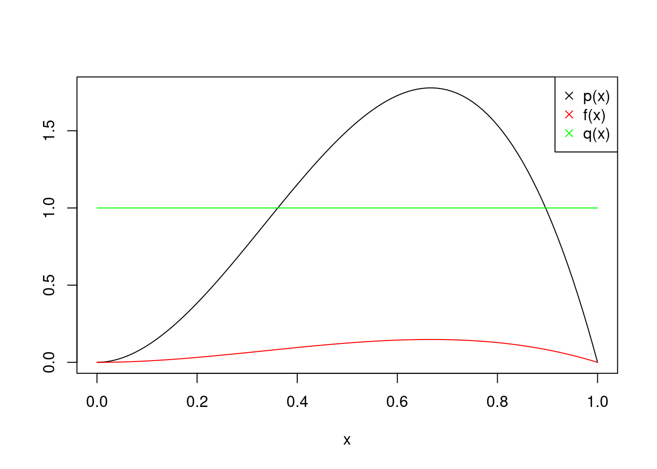
Figure 11.1: Visualizing Our Three Functions

Note that this algorithm allows for other proposal distributions. The only requirement of a proposal distribution is that its range of possible values must subsume the range of possible values of the target.

Write a function called arSamp(n) that samples from $p (x)$ using accept-reject sampling. It should take a single argument that is equal to the number of samples desired. Below is one step of the accept-reject algorithm. You will need to do many iterations of this. The number of iterations will be random, because some of these proposals will not be accepted.

Algorithm 1: Accept-Reject Sampling (One Step)

Find $M$ such that $M > \frac{f (x)}{q (x)}$ for all possible $x$ (the smaller the better).
Sample $X$ from $q (x)$ .
Sample $Y ∣ X$ from $Bernoulli (\frac{f (X)}{q (X) M})$ .
If $Y = 1$ , then return $X$ .
Otherwise, return nothing.

Write a function called multiplyTwoMats(A,B) that performs matrix multiplication. It should take two matrix arguments: A and B. Then it should return the matrix product AB. Use two nested for loops to write this function. Make sure to test this function against the usual tool you use to multiply matrices together: %*%.

Suppose you are trying to predict a value of $Y$ given some information about a corresponding independent variable $x$ . Suppose further that you have a historical data set of observations $(x_{1}, y_{1}), \dots, (x_{n}, y_{n})$ . One approach for coming up with predictions is to use Nadaraya–Watson Kernel Regression (Nadaraya 1964) (Watson 1964). The prediction this approach provides is simply a weighted average of all of the historically-observed data points $y_{1}, \dots, y_{n}$ . The weight for a given $y_{i}$ will be larger if $x_{i}$ is “close” to the value $x$ that you are obtaining predictions for. On the other hand, if $x_{j}$ is far away from $x$ , then the weight for $y_{j}$ will be relatively small, and so this data point won’t influence the prediction much.

Write a function called kernReg(xPred,xData,yData,kernFunc) that computes the Nadaraya–Watson estimate of the prediction of $Y$ given $X = x$ . Do not use a for loop in your function definition. The formula is $\sum_{i = 1}^{n} \frac{K (x - x_{i})}{\sum_{j = 1}^{n} K (x - x_{j})} y_{i},$ where $x$ is the point you’re trying to get a prediction for.

Your function should return one floating point number.
The input xPred will be a floating point number.
The input xData is a one-dimensional vector of numerical data of independent variables.
The input yData is a one-dimensional vector of numerical data of dependent variables.
kernFunc is a function that accepts a numeric vector and returns a floating point. It’s vectorized.

Below is some code that will help you test your predictions. The kernel function, gaussKernel(), implements the Gaussian kernel function $K (z) = \exp [- z^{2} / 2] / \sqrt{2 π}$ . Notice the creation of preds was commented out. Use a for loop to generate predictions for all elements of xTest and store them in the vector preds.

gaussKernel <- dnorm
xTest <- seq(0,10,length.out= 100)
yTest <- xTest*2 
# preds <- ?
plot(xTest, yTest, type = "b")
lines(xTest, preds, col = "red")

11.3.2 Python Questions

Suppose you go to the casino with $10$ dollars. You decide that your policy is to play until you go broke, or until you triple your money. The only game you play costs $$ 1$ to play. If you lose, you lose that dollar. If you win, you get another $$ 1$ in addition to getting your money back.

Write a function called sim_night(p) that simulates your night of gambling. Have it return a Pandas Series with the running balance of money you have over the course of a night. For example, if you lose $10$ games in a row, and go home early, the returned Series contains $9, \dots, 1, 0$ . This function will only take one input, p, which is the probability of winning any/every game you play.
Use a for loop to call your function $5000$ times with probability p=.5. Each time, store the number of games played. Store them all in a Numpy array or Pandas Series called simulated_durations.
Take the average of simulated_durations. This is your Monte Carlo estimate of the expected duration. How does it compare with what you think it should be theoretically?
Perform the same analysis to estimate the expected duration when $p = .7$ . Store your answer as a float called expec_duration.

Suppose you have the following data set. Please include the following snippet in your submission.

import numpy as np
import pandas as pd
my_data = pd.read_csv("sim_data.csv", header=None).values.flatten()

This question will demonstrate how to implement The Bootstrap (Efron 1979), which is a popular nonparametric approach to understand the distribution of a statistic of interest. The main idea is to calculate your statistic over and over again on bootstrapped data sets, which are data sets randomly chosen, with replacement, from your original data set my_data. Each bootstrapped data set is of the same size as the original data set, and each bootstrapped data set will yield one statistic. Collect all of these random statistics, and it is a good approximation to the statistic’s theoretical distribution.

Calculate the mean of this data set and store it as a floating point number called sample_mean.
Calculate $5, 000$ bootstrap sample means. Store them in a Numpy array called bootstrapped_means. Use a for loop, and inside the loop, sample with replacement $1000$ times from the length $1000$ data set. You can use the function np.random.choice() to accomplish this.
Calculate the sample mean of these bootstrapped means. This is a good estimate of the theoretical mean/expectation of the sample mean. Call it mean_of_means.
Calculate the sample variance of these bootstrapped means. This is a good estimate of the theoretical variance of the sample mean. Call it var_of_means.

Write a function called ar_samp(n) that samples from $p (x)$ using accept-reject sampling. Use any proposal distribution that you’d like. It should take a single argument that is equal to the number of samples desired. Sample from the following target: $p (x) \propto f (x) := \exp [\cos (2 π x)] x^{2} (1 - x), 0 < x < 1.$

References

Efron, B. 1979. “Bootstrap Methods: Another Look at the Jackknife.” The Annals of Statistics 7 (1): 1–26. https://doi.org/10.1214/aos/1176344552.

Lutz, Mark. 2013. Learning Python. 5th ed. Beijing: O’Reilly. https://www.safaribooksonline.com/library/view/learning-python-5th/9781449355722/.

Nadaraya, E. A. 1964. “On Estimating Regression.” Theory of Probability & Its Applications 9 (1): 141–42. https://doi.org/10.1137/1109020.

Watson, Geoffrey S. 1964. “Smooth Regression Analysis.” Sankhyā: The Indian Journal of Statistics, Series A (1961-2002) 26 (4): 359–72. http://www.jstor.org/stable/25049340.

This is the density of a $Beta (3, 2)$ random variable, if you’re curious.↩