Chapter 14 An Introduction to Object-Oriented Programming
Object-Oriented Programming (OOP) is a way of thinking about how to organize programs. This way of thinking focuses on objects. In the next chapter, we focus on organizing programs by functions, but for now we stick to objects. We already know about objects from the last chapter, so what’s new here?
The difference is that we’re creating our own types now. In the last chapter we learned about built-in types: floating point numbers, lists, arrays, functions, etc. Now we will discuss broadly how one can create his own types in both R and Python. These user-defined types can be used as cookie cutters. Once we have the cookie cutter, we can make as many cookies as we want!
We will not go into this too deeply, but it is important to know how how code works so that we can use it more effectively. For instance, in Python, we frequently write code like my_data_frame.doSomething(). The material in this chapter will go a long way to describe how we can make our own types with custom behavior.
Here are a few abstract concepts that will help thinking about OOP. They are not mutually exclusive, and they aren’t unique to OOP, but understanding these words will help you understand the purpose of OOP. Later on, when we start looking at code examples, I will alert you to when these concepts are coming into play.
Composition refers to the idea when one type of object contains an object of another type. For example, a linear model object could hold on to estimated regression coefficients, residuals, etc.
Inheritance takes place when an object can be considered to be of another type(s). For example, an analysis of variance linear regression model might be a special case of a general linear model.
Polymorphism is the idea that the programmer can use the same code on objects of different types. For example, built-in functions in both R and Python can work on arguments of a wide variety of different types.
Encapsulation is another word for complexity hiding. Do you have to understand every line of code in a package you’re using? No, because a lot of details are purposefully hidden from you.
Modularity is an idea related to encapsulation–it means splitting something into independent pieces. How you split code into different files, different functions, different classes–all of that has to do with modularity. It promotes encapsulation, and it allows you to think about only a few lines of code at a time.
The interface, between you and the code you’re using, describes what can happen, but not how it happens. In other words, it describes some functionality so that you can decide whether you want to use it, but there are not enough details for you to make it work yourself. For example, all you have to do to be able to estimate a complicated statistical model is to look up some documentation.23 In other words, you only need to be familiar with the interface, not the implementation.
The implementation of some code you’re using describes how it works in detail. If you are a package author, you can change your code’s implementation “behind the scenes” and ideally, your end-users would never notice.
14.1 OOP In Python
14.1.1 Overview
In Python, classes are user-defined types. When you define your own class, you describe what kind of information it holds onto, and how it behaves.
To define your own type, use the class keyword. Objects created with a user-defined class are sometimes called instances. They behave according to the rules written in the class definition–they always have data and/or functions bundled together in the same way, but these instances do not all have the same data.
To be more clear, classes may have the following two things in their definition.
Attributes (aka data members) are pieces of data “owned” by an instance created by the class.
(Instance) methods are functions “owned” by an instance created by the class. They can use and/or modify data belonging to the class.
14.1.2 A First Example
Here’s a simple example. Say we are interested in calculating, from numerical data \(x_1, \ldots, x_n\), a sample mean: \[\begin{equation} \bar{x}_n = \frac{\sum_{i=1}^n x_i}{n}. \end{equation}\]
In Python, we can usually calculate this one number very easily using np.average. However, this function requires that we pass into it all of the data at once. What if we don’t have all the data at any given time? In other words, suppose that the data arrive intermittently
.
We might consider taking advantage of a recursive formula for the sample means.
\[\begin{equation} \bar{x}_n = \frac{(n-1) \bar{x}_{n-1} + x_n}{n} \end{equation}\]
How would we program this in Python? A first option: we might create a variable my_running_ave, and after every data point arrives, we could
my_running_ave = 1.0
my_running_ave
## 1.0
my_running_ave = ((2-1)*my_running_ave + 3.0)/2
my_running_ave
## 2.0
my_running_ave = ((3-1)*my_running_ave + 2.0)/3
my_running_ave
## 2.0
There are a few problems with this. Every time we add a data point, the formula slightly changes. Every time we update the average, we have to write a different line of code. This opens up the possibility for more bugs, and it makes your code less likely to be used by other people and more difficult to understand. And if we were trying to code up something more complicated than a running average? That would make matters even worse.
A second option: write a class that holds onto the running average, and that has
- an
updatemethod that updates the running average every time a new data point is received, and - a
get_current_xbarmethod that gets the most up-to-date information for us.
Using our code would look like this:
my_ave = RunningMean() # create running average object
my_ave.get_current_xbar() # no data yet!
my_ave.update(1.) # first data point
my_ave.get_current_xbar() # xbar_1
## 1.0
my_ave.update(3.)  # second data point
my_ave.get_current_xbar()  #xbar_2
## 2.0
my_ave.n   # my_ave.n instead of self.n
## 2
There is a Python convention that stipules class names should be written in UpperCamelCase (e.g. RunningMean).
That’s much better! Notice the encapsulation–while looking at this code we do not need to think about the mathematical formula that is used to process the data. We only need to type in the correct data being used. In other words, the implementation is separated from the interface. The interface in this case, is just the name of the class methods, and the arguments they expect. That’s all we need to know about to use this code.
After seeing these new words that are unfamiliar and long, it’s tempting to dismiss these new ideas as superfluous. After all, if you are confident that you can get your program working, why stress about all these new concepts? If it ain’t broke, don’t fix it, right?
I urge you to try to keep an open mind, particularly if you are already confident that you understand the basics of programming in R and Python. The topics in this chapter are more centered around design choices. This material won’t help you write a first draft of a script even faster, but it will make your code much better. Even though you will have to slow down a bit before you start typing, thinking about your program more deeply will prevent bugs and allow more people to use your code.
Classes (obviously) need to be defined before they are used, so here is the definition of our class.
class RunningMean:
    """Updates a running average"""
    def __init__(self):
        self.current_xbar = 0.0
        self.n = 0
    def update(self, new_x):
        self.n += 1
        self.current_xbar *= (self.n-1)
        self.current_xbar += new_x
        self.current_xbar /= self.n
    def get_current_xbar(self):
        if self.n == 0:
            return None
        else:
            return self.current_xbar
Methods that look like __init__, or that possess names that begin and end with two underscores, are called dunder (double underscore) methods, special methods or magic methods. There are many that you can take advantage of! For more information see this.
Here are the details of the class definition:
Defining class methods looks exactly like defining functions! The primary difference is that the first argument must be
self. If the definition of a method refers toself, then this allows the class instance to refer to its own (heretofore undefined) data attributes. Also, these method definitions are indented inside the definition of the class.This class owns two data attributes. One to represent the number of data points seen up to now (
n), and another to represent the current running average (current_xbar).- Referring to data members requires dot notation.
self.nrefers to thenbelonging to any instance. This data attribute is free to vary between all the objects instantiated by this class. The
__init__method performs the setup operations that are performed every time any object is instantiated.The
updatemethod provides the core functionality using the recursive formula displayed above.get_current_xbarsimply returns the current average. In the case that this function is called before any data has been seen, it returnsNone.
A few things you might find interesting:
Computationally, there is never any requirement that we must hold all of the data points in memory. Our data set could be infinitely large, and our class will hold onto only one floating point number, and one integer.
This example is generalizable to other statistical methods. In a mathematical statistics course, you will learn about a large class of models having sufficient statistics. Most sufficient statistics have recursive formulas like the one above. Second, many algorithms in time series analysis have recursive formulas and are often needed to analyze large streams of data. They can all be wrapped into a class in a way that is similar to the above example.
14.1.3 Adding Inheritance
How can we use inheritance in statistical programming? A primary benefit of inheritance is code re-use, so one example of inheritance is writing a generic algorithm as a base class, and a specific algorithm as a class that inherits from the base class. For example, we could re-use the code in the RunningMean class in a variety of other classes.
Let’s make some assumptions about a parametric model that is generating our data. Suppose I assume that the data points \(x_1, \ldots, x_n\) are a “random sample”24 from a normal distribution with mean \(\mu\) and variance \(\sigma^2=1\). \(\mu\) is assumed to be unknown (this is, after all, and interval for \(\mu\)), and \(\sigma^2\) is assumed to be known, for simplicity.
A \(95\%\) confidence interval for the true unknown population mean \(\mu\) is
\[\begin{equation} \left( \bar{x} - 1.96 \sqrt{\frac{\sigma^2}{n}}, \bar{x} + 1.96 \sqrt{\frac{\sigma^2}{n}} \right). \end{equation}\]
The width of the interval shrinks as we get more data (as \(n \to \infty\)). We can write another class that, not only calculates the center of this interval, \(\bar{x}\), but also returns the interval endpoints.
If we wrote another class from scratch, then we would need to rewrite a lot of the code that we already have in the definition of RunningMean. Instead, we’ll use the idea of inheritance.
import numpy as np

class RunningCI(RunningMean):# <-notice what's inside the parentheses
    """Updates a running average and
    gives you a known-variance confidence interval"""

    def __init__(self, known_var):
        super().__init__()
        self.known_var = known_var

    def get_current_interval(self):
        if self.n == 0:
            return None
        else:
            half_width = 1.96 * np.sqrt(self.known_var / self.n)
            left_num = self.current_xbar - half_width
            right_num = self.current_xbar + half_width
            return np.array([left_num, right_num])
The parentheses in the first line of the class definition signal that this new class definition is inheriting from RunningMean. Inside the definition of this new class, when I refer to self.current_xbar Python knows what I’m referring to because it is defined in the base class. Last, I am using super() to access the base class’s methods, such as __init__.
my_ci = RunningCI(1) # create running average object
my_ci.get_current_xbar() # no data yet!
my_ci.update(1.)
my_ci.get_current_interval()
## array([-0.96,  2.96])
my_ci.update(3.)
my_ci.get_current_interval()
## array([0.61407071, 3.38592929])
This example also demonstrates polymorphism. Polymorphism comes from the Greek for “many forms.” “Forms” means “type” or “class” in this case. If the same code (usually a function or method) works on objects of different types, that’s polymorphic. Here, the update method worked on an object of class RunningCI, as well as an object of RunningMean.
Why is this useful? Consider this example.
Inside the inner for loop, there is no need for include conditional logic that tests for what kind of type each thing is. We can iterate through time more succinctly.
for datum in time_series:
    for thing in obj_list:
        if isinstance(thing, class1):
            thing.updatec1(xt)
        if isinstance(thing, class2):
            thing.updatec2(xt)
        if isinstance(thing, class3):
            thing.updatec3(xt)
        if isinstance(thing, class4):
            thing.updatec4(xt)
        if isinstance(thing, class5):
            thing.updatec5(xt)
        if isinstance(thing, class6):
            thing.updatec6(xt)
If, in the future, you add a new class called class7, then you need to change this inner for loop, as well as provide new code for the class.
14.1.4 Adding in Composition
Composition also enables code re-use. Inheritance ensures an “is a” relationship between base and derived classes, and composition promotes a “has a” relationship. Sometimes it can be tricky to decide which technique to use, especially when it comes to statistical programming.
Regarding the example above, you might argue that a confidence interval isn’t a particular type of a sample mean. Rather, it only has a sample mean. If you believe this, then you might opt for a composition based model instead. With composition, the derived class (the confidence interval class) will be decoupled from the base class (the sample mean class). This decoupling will have a few implications. In general, composition is more flexible, but can lead to longer, uglier code.
You will lose polymorphism.
Your code might become less re-usable.
You have to write any derive class methods you want because you don’t inherit any from the base class. For example, you won’t automatically get the
.update()or the.get_current_xbar()method for free. This can be tedious if there are a lot of methods you want both classes to have that should work the same exact way for both classes. If there are, you would have to re-write a bunch of method definitions.On the other hand, this could be good if you have methods that behave completely differently. Each method you write can have totally different behavior in the derived class, even if the method names are the same in both classes. For instance,
.update()could mean something totally different in these two classes. Also, in the derive class, you can still call the base class’s.update()method.
Many-to-one relationships are easier. It’s generally easier to “own” many base class instances rather than inherit from many base classes at once. This is especially true if this is the only book on programming you plan on reading–I completely avoid the topic of multiple inheritance!
Sometimes it is very difficult to choose between using composition or using inheritance. However, this choice should be made very carefully. If you make the wrong one, and realize too late, refactoring your code might be very time consuming!
Here is an example implementation of a confidence interval using composition. Notice that this class “owns” a RunningMean instance called self.mean. This is contrast with inheriting from the RunningMean class.
class RunningCI2:
    """Updates a running average and
    gives you a known-variance confidence interval"""

    def __init__(self, known_var):
        self.mean = RunningMean()
        self.known_var = known_var

    def update(self, new_x):
        self.mean.update(new_x)

    def get_current_interval(self):
        if self.n == 0:
            return None
        else:
            half_width = 1.96 * np.sqrt(self.known_var / self.n)
            left = self.mean.get_current_xbar() - half_width
            right = self.mean.get_current_xbar() + half_width
            return np.array([left, right])
14.2 OOP In R
R, unlike Python, has many different kinds of classes. In R, there is not only one way to make a class. There are many! I will discuss
- S3 classes,
- S4 classes,
- Reference classes, and
- R6 classes.
If you like how Python does OOP, you will like reference classes and R6 classes, while S3 and S4 classes will feel strange to you.
It’s best to learn about them chronologically, in my opinion. S3 classes came first, S4 classes sought to improve upon those. Reference classes rely on S4 classes, and R6 classes are an improved version of Reference classes (Wickham 2014).
14.2.1 S3 objects: The Big Picture
With S3 (and S4) objects, calling a method print() will not look like this.
my_obj.print()Instead, it will look like this:
print(my_obj)The primary goal of S3 is polymorphism (Grolemund 2014). We want functions like print(), summary() and plot() to behave differently when objects of a different type are passed in to them. Printing a linear model should look a lot different than printing a data frame, right? So we can write code like the following, we only have to remember fewer functions as an end-user, and the “right” thing will always happen. If you’re writing a package, it’s also nice for your users that they’re able to use the regular functions that they’re familiar with. For instance, I allow users of my package cPseudoMaRg (Brown 2021) to call print() on objects of type cpmResults. In section 13.2, ggplot2 instances, which are much more complicated than plain numeric vectors, are +ed together.
# print works on pretty much everything
print(myObj)
print(myObjOfADifferentClass)
print(aThirdClassObject)
This works because these “high-level” functions (such as print()), will look at its input and choose the most appropriate function to call, based on what kind of type the input has. print() is the high-level function. When you run some of the above code, it might not be obvious which specific function print() chooses for each input. You can’t see that happening, yet.
Last, recall that this discussion only applies to S3 objects. Not all objects are S3 objects, though. To find out if an object x is an S3 object, use is.object(x).
14.2.2 Using S3 objects
Using S3 objects is so easy that you probably don’t even know that you’re actually using them. You can just try to call functions on objects, look at the output, and if you’re happy with it, you’re good. However, if you’ve ever asked yourself: “why does print() (or another function) do different things all the time?” then this section will be useful to you.
print() is a generic function which is a function that looks at the type of its first argument, and then calls another, more specialized function depending on what type that argument is. Not all functions in R are generic, but some are. In addition to print(), summary() and plot() are the most ubiquitous generic functions. Generic functions are an interface, because the user does not need to concern himself with the details going on behind the scenes.
In R, a method is a specialized function that gets chosen by the generic function for a particular type of input. The method is the implementation. When the generic function chooses a particular method, this is called method dispatch.
If you look at the definition of a generic function, let’s take plot() for instance, it has a single line that calls UseMethod().
## function (x, y, ...)
## UseMethod("plot")
## <bytecode: 0x5654afa2fd00>
## <environment: namespace:base>
UseMethod() performs method dispatch. Which methods can be dispatched to? To see that, use the methods() function.
## [1] 39All of these S3 class methods share the same naming convention. Their name has the generic function’s name as a prefix, then a dot (.), then the name of the class that they are specifically written to be used with.
R’s dot-notation is nothing like Python’s dot-notation! In R, functions do not belong to types/classes like they do in Python!
Method dispatch works by looking at the class attribute of an S3 object argument. An object in R may or may not have a set of attributes, which are a collection of name/value pairs that give a particular object extra functionality. Regular vectors in R don’t have attributes (e.g. try running attributes(1:3)), but objects that are “embellished” versions of a vector might (e.g. run attributes(factor(1:3))). Attributes in R are similar to attributes in Python, but they are usually only used as “tags” to elicit some sort of behavior when the object is passed into a function.
class() will return misleading results if it’s called on an object that isn’t an S3 object. Make sure to check with is.object() first.
Also, these methods are not encapsulated inside a class definition like they are in Python, either. They just look like loose functions–the method definition for a particular class is not defined inside the class. These class methods can be defined just as ordinary functions, out on their own, in whatever file you think is appropriate to define functions in.
As an example, let’s try to plot() some specific objects.
aDF <- data.frame(matrix(rnorm(100), nrow = 10))
is.object(aDF) # is this s3?
## [1] TRUE
class(aDF)
## [1] "data.frame"
plot(aDF)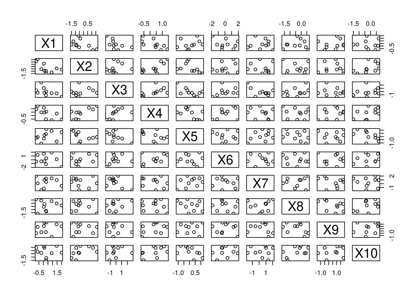
Figure 14.1: A Scatterplot Matrix
Because aDF has its class set to data.frame, this causes plot() to try to find a plot.data.frame() method. If this method was not found, R would attempt to find/use a plot.default() method. If no default method existed, an error would be thrown.
As another example, we can play around with objects created with the ecdf() function. This function computes an empirical cumulative distribution function, which takes a real number as an input, and outputs the proportion of observations that are less than or equal to that input25.
myECDF <- ecdf(rnorm(100))
is.object(myECDF)
## [1] TRUE
class(myECDF)
## [1] "ecdf"     "stepfun"  "function"
plot(myECDF)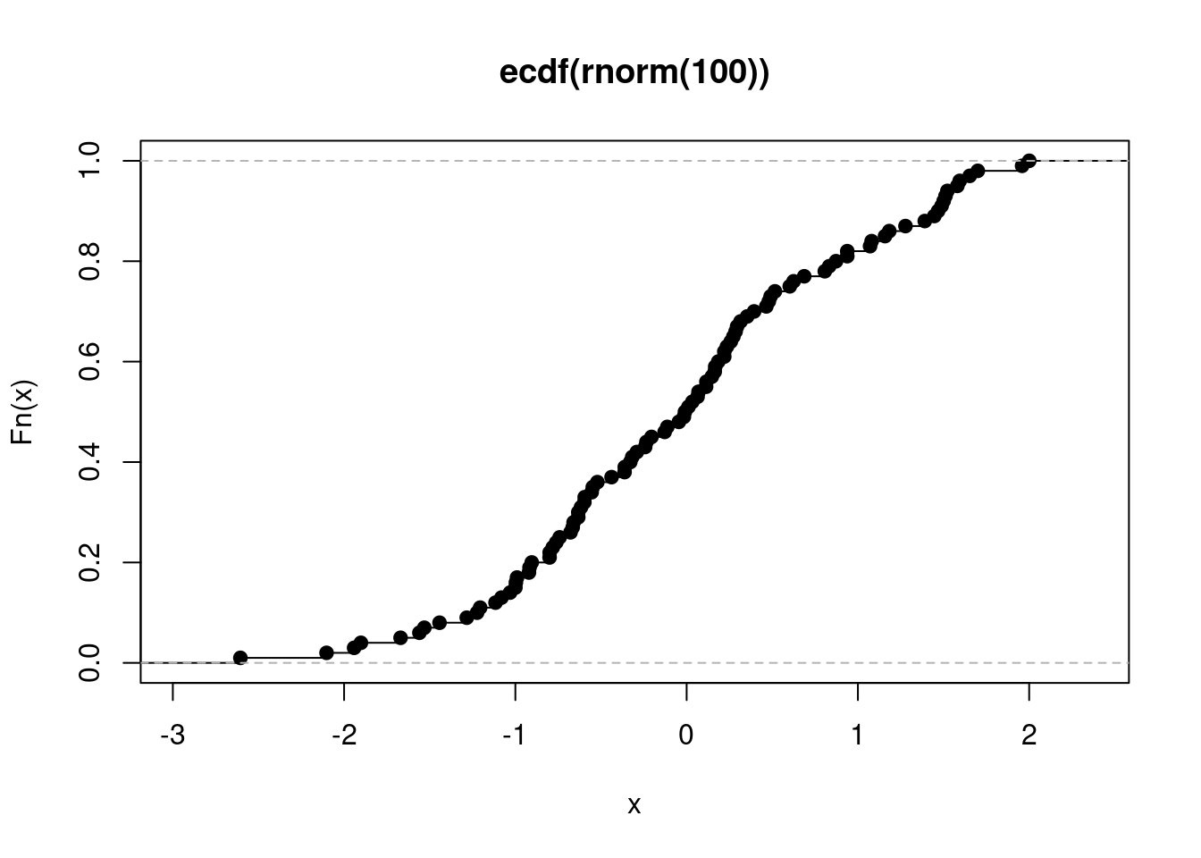
Figure 14.2: Plotting an Empirical Cumulative Distribution Function
This is how inheritance works in S3. The ecdf class inherits from the stepfun class, which in turn inherits from the function class. When you call plot(myECDF), ultimately plot.ecdf() is used on this object. However, if plot.ecdf() did not exist, plot.stepfun() would be tried. S3 inheritance in R is much simpler than Python’s inheritance!
14.2.3 Creating S3 objects
Creating an S3 object is very easy, and is a nice way to spruce up some bundled up object that you’re returning from a function, say. All you have to do is tag an object by changing its class attribute. Just assign a character vector to it!
Here is an example of creating an object of CoolClass.
myThing <- 1:3
attributes(myThing)
## NULL
class(myThing) <- "CoolClass"
attributes(myThing) # also try class(myThing)
## $class
## [1] "CoolClass"
myThing is now an instance of CoolClass, even though I never defined what a CoolClass was ahead of time! If you’re used to Python, this should seem very strange. Compared to Python, this approach is very flexible, but also, kind of dangerous, because you can change the classes of existing objects. You shouldn’t do that, but you could if you wanted to.
After you start creating your own S3 objects, you can write your own methods associated with these objects. That way, when a user of your code uses typical generic functions, such as summary(), on your S3 object, you can control what interesting things will happen to the user of your package. Here’s an example.
summary(myThing)
## [1] "No summary available!"
## [1] "Cool Classes are too cool for summaries!"
## [1] ":)"
The summary() method I wrote for this class is the following.
summary.CoolClass <- function(object,...){
  print("No summary available!")
  print("Cool Classes are too cool for summaries!")
  print(":)")
}
When writing this, I kept the signature the same as summary()’s.
14.2.4 S4 objects: The Big Picture
S4 was developed after S3. If you look at your search path (type search()), you will see package:methods. That’s where all the code you need to do S4 is. Here are the similarities and differences between S3 and S4.
- They both use generic functions and methods work in the same way.
- Unlike in S3, S4 classes allow you to use multiple dispatch, which means the generic function can dispatch on multiple arguments, instead of just the first argument.
- S4 class definitions are strict–they aren’t just name tags like in S3.
- S4 inheritance feels more like Python’s. You can think of a base class object living inside a child class object.
- S4 classes can have default data members via
prototypes.
Much more information about S4 classes can be obtained by reading Chapter 15 in Hadley Wickham’s book.
14.2.5 Using S4 objects
One CRAN package that uses S4 is the Matrix package. Here is a short and simple code example.
S4 objects are also extremely popular in packages hosted on Bioconductor. Bioconductor is similar to CRAN, but its software has a much more specific focus on bioinformatics. To download packages from Bioconductor, you can check out the installation instructions provided here.
library(Matrix)
M <- Matrix(10 + 1:28, 4, 7)
isS4(M)
## [1] TRUE
M
## 4 x 7 Matrix of class "dgeMatrix"
##      [,1] [,2] [,3] [,4] [,5] [,6] [,7]
## [1,]   11   15   19   23   27   31   35
## [2,]   12   16   20   24   28   32   36
## [3,]   13   17   21   25   29   33   37
## [4,]   14   18   22   26   30   34   38
M@Dim
## [1] 4 7
Inside an S4 object, data members are called slots, and they are accessed with the @ operator (instead of the $ operator). Objects can be tested if they are S4 with the function isS4(). Otherwise, they look and feel just like S3 objects.
14.2.6 Creating S4 objects
Here are the key takeaways:
- create a new S4 class with
setClass(), - create a new S4 object with
new(), - S4 classes have a fixed amount of slots, a name, and a fixed inheritance structure.
Let’s do an example that resembles the example we did in Python, where we defined a RunningMean class and a RunningCI class.
setClass("RunningMean",
         slots = list(n = "integer",
                      currentXbar = "numeric"))
setClass("RunningCI",
         slots = list(knownVar = "numeric"),
         contains = "RunningMean")
Here, unlike in S3 class’s, we actually have to define a class with setClass(). In the parlance of S4, slots= are a class’ data members, and contains= signals that one class inherits from another (even though “contains” kind of sounds like it’s suggesting composition).
New objects can be created with the new() function after this is accomplished.
new("RunningMean", n = 0L, currentXbar = 0)
new("RunningCI", n = 0L, currentXbar = 0, knownVar = 1.0)
Next we want to define an update() generic function that will work on objects of both types. This is what gives us polymorphism . The generic update() will call specialized methods for objects of class RunningMean and RunningCI.
Recall that in the Python example, each class had its own update method. Here, we still have a specialized method for each class, but S4 methods don’t have to be defined inside the class definition, as we can see below.
## Creating a new generic function for 'update' in the global environment
## [1] "update"setGeneric("update", function(oldMean, newNum) {
standardGeneric("update")
})
setMethod("update",
c(oldMean = "RunningMean", newNum = "numeric"),
function(oldMean, newNum) {
oldN <- oldMean@n
oldAve <- oldMean@currentXbar
newAve <- (oldAve*oldN + newNum)/(oldN + 1)
newN <- oldN + 1L
return(new("RunningMean", n = newN, currentXbar = newAve))
}
)
setMethod("update",
c(oldMean = "RunningCI", newNum = "numeric"),
function(oldMean, newNum) {
oldN <- oldMean@n
oldAve <- oldMean@currentXbar
newAve <- (oldAve*oldN + newNum)/(oldN + 1)
newN <- oldN + 1L
return(new("RunningCI", n = newN, currentXbar = newAve,
knownVar = oldMean@knownVar))
}
)Here’s a demonstration of using these two classes that mirrors the example in subsection 14.1.3
myAve <- new("RunningMean", n = 0L, currentXbar = 0)
myAve <- update(myAve, 3)
myAve
## An object of class "RunningMean"
## Slot "n":
## [1] 1
##
## Slot "currentXbar":
## [1] 3
myAve <- update(myAve, 1)
myAve
## An object of class "RunningMean"
## Slot "n":
## [1] 2
##
## Slot "currentXbar":
## [1] 2

myCI <- new("RunningCI", n = 0L, currentXbar = 0, knownVar = 1.0)
myCI <- update(myCI, 3)
myCI
## An object of class "RunningCI"
## Slot "knownVar":
## [1] 1
##
## Slot "n":
## [1] 1
##
## Slot "currentXbar":
## [1] 3
myCI <- update(myCI, 1)
myCI
## An object of class "RunningCI"
## Slot "knownVar":
## [1] 1
##
## Slot "n":
## [1] 2
##
## Slot "currentXbar":
## [1] 2
This looks more functional (more information on functional programming is available in chapter 15) than the Python example because the update() function does not change an object with a side effect. Instead, it takes the old object, changes it, returns the new object, and uses assignment to overwrite the object. The benefit of this approach is that the assignment operator (<-) signals to us that something is changing. However, there is more data copying involved, so the program is presumably slower than it needs to be.
The big takeaway here is that S3 and S4 don’t feel like Python’s encapsulated OOP. If we wanted to write stateful programs, we might consider using Reference Classes, or R6 classes.
14.2.7 Reference Classes: The Big Picture
Reference Classes are built on top of S4 classes, and were released in late 2010. They feel very different from S3 and S4 classes, and they more closely resemble Python classes, because
- their method definitions are encapsulated inside class definitions like in Python, and
- the objects they construct are mutable.
So it will feel much more like Python’s class system. Some might say using reference classes that will lead to code that is not very R-ish, but it can be useful for certain types of programs (e.g. long-running code, code that that performs many/high-dimensional/complicated simulations, or code that circumvents storing large data set in your computer’s memory all at once).
14.2.8 Creating Reference Classes
Creating reference classes is done with the function setRefClass. I create a class called RunningMean that produces the same behavior as that in the previous example.
RunningMeanRC <- setRefClass("RunningMeanRC",
                             fields = list(current_xbar = "numeric",
                                           n = "integer"),
                             methods = list(
                               update = function(new_x){
                                 n <<- n + 1L
                                 new_sum <- current_xbar*(n-1) + new_x
                                 current_xbar <<- new_sum/n
                                }))
This tells us a few things. First, data members are called fields now. Second, changing class variables is done with the <<-. We can use it just as before.
my_ave <- RunningMeanRC$new(current_xbar=0, n=0L)
my_ave
## Reference class object of class "RunningMeanRC"
## Field "current_xbar":
## [1] 0
## Field "n":
## [1] 0
my_ave$update(1.)
my_ave$current_xbar
## [1] 1
my_ave$n
## [1] 1
my_ave$update(3.)
my_ave$current_xbar
## [1] 2
my_ave$n
## [1] 2
Compare how similar this code looks to the code in 14.1.2! Note the paucity of assignment operators, and plenty of side effects.
14.2.9 Creating R6 Classes
I quickly implement the above example as an R6 class. A more detailed introduction to R6 classes is provided in the vignette from the package authors.
You’ll notice the reappearance of the self keyword. R6 classes have a self keyword just like in Python. They are similar to reference classes, but there are a few differences:
- they have better performance than reference classes, and
- they don’t make use of the
<<-operator.
library(R6)

RunningMeanR6 <- R6Class("RunningMeanR6",
                  public = list(
                    current_xbar = NULL,
                    n = NULL,
                    initialize = function(current_xbar = NA, n = NA) {
                      self$current_xbar <- current_xbar
                      self$n <- n
                    },
                    update = function(new_x) {
                      newSum <- self$current_xbar*self$n + new_x
                      self$n <- self$n + 1L
                      self$current_xbar <- newSum / self$n
                    }
                  )
)
my_r6_ave <- RunningMeanR6$new(current_xbar=0, n=0L)
my_r6_ave
## <RunningMeanR6>
##   Public:
##     clone: function (deep = FALSE)
##     current_xbar: 0
##     initialize: function (current_xbar = NA, n = NA)
##     n: 0
##     update: function (new_x)
my_r6_ave$update(1.)
my_r6_ave$current_xbar
## [1] 1
my_r6_ave$n
## [1] 1
my_r6_ave$update(3.)
my_r6_ave$current_xbar
## [1] 2
my_r6_ave$n
## [1] 2
14.3 Exercises
14.3.1 Python Questions
If you are interested in estimating a linear regression model, there is a LinearRegression class that you might consider using in the sklearn.linear_model submodule. In this lab, we will create something similar, but a little more simplified.
A simple linear regression model will take in \(n\) independent variables \(x_1, \ldots, x_n\), and \(n\) dependent variables \(y_1, \ldots, y_n\), and try to describe their relationship with a function: \[\begin{equation} y_i = \beta_0 + \beta_1 x_i + \epsilon_i. \end{equation}\] The coefficients \(\beta_0\) and \(\beta_1\) are unknown, and so must be estimated with the data. Estimating the variance of the noise terms \(\epsilon_i\) may also be of interest, but we do not concern ourselves with that here.
The formulas for the estimated slope (i.e. \(\hat{\beta}_1\)) and the estimated intercept (i.e. \(\hat{\beta}_0\)) are as follows: \[\begin{equation} \hat{\beta}_1 = \frac{\sum_{i=1}^n (x_i - \bar{x})(y_i-\bar{y)}}{\sum_{j=1}^n (x_j - \bar{x})^2} \end{equation}\]
\[\begin{equation} \hat{\beta}_0 = \bar{y} - \hat{\beta}_1\bar{x}. \end{equation}\]
Create a class that performs simple linear regression.
- Name it
SimpleLinReg. - Its
.__init__()method should not take any additional parameters. It should set two data attributes/membersest_interceptandest_slope, tonp.nan. - Give it a
.fit()method that takes in two 1-dimensional Numpy arrays. The first should be the array of independent values, and the second should be the set of dependent values. .fit(x,y)should notreturnanything, but it should store two data attributes/members:est_interceptandest_slope. Every time.fit()is called, it will re-calculate the coefficient/parameter estimates.- Give it a
.get_coeffs()method. It should not make any changes to the data attributes/members of the class. It should simplyreturna Numpy array with the parameter estimates inside. Make the first element the estimated intercept, and the second element the estimated slope. If no such coefficients have been estimated at the time of its calling, it should return the same size array but with the initialnp.nans inside.
After you’ve finished writing your first class, you can bask in the glory and run the following test code:
mod = SimpleLinReg()
mod.get_coeffs()
x = np.arange(10)
y = 1 + .2 * x + np.random.normal(size=10)
mod.fit(x,y)
mod.get_coeffs()
Reconsider the above question that asked you to write a class called SimpleLinReg.
- Write a new class called
LinearRegression2that preserves all of the existing functionality ofSimpleLinReg. Do this in a way that does not excessively copy and paste code fromSimpleLinReg. - Give your new class a method called
.visualize()that takes no arguments and plots the most recent data, the data most recently provided to.fit(), in a scatterplot with the estimated regression line superimposed. - Unfortunately,
SimpleLinReg().fit(x,y).get_coeffs()will not return estimated regression coefficients. Give your new class this functionality. In other words, makeLinearRegression2().fit(x,y).get_coeffs()spit out regression coefficients. Hint: the solution should only require one extra line of code, and it should involve theselfkeyword.
Consider the following time series model (West and Harrison 1989) \[\begin{equation} y_t = \beta_t + \epsilon_t \\ \beta_t = \beta_{t-1} + w_t \\ \beta_1 = w_1 \end{equation}\] Here \(y_t\) is observed time series data, each \(\epsilon_t\) is measurement noise with variance \(V\) and each \(w_t\) is also noise but with variance \(W\). Think of \(\beta_t\) as a time-varying regression coefficient.
Imagine our data are arriving sequentially. The Kalman Filter (Kalman 1960) cite provides an “optimal” estimate of each \(\beta_t\) given all of the information we have up to time \(t\). What’s better is that the algorithm is recursive. Future estimates of \(\beta_t\) will be easy to calculate given our estimates of \(\beta_{t-1}\).
Let’s call the mean of \(\beta_{t-1}\) (given all the information up to time \(t-1\)) \(m_{t-1}\), and the variance of \(\beta_{t-1}\) (given all the information up to time \(t-1\)) \(P_{t-1}\). Then the Kalman recursions for this particular model are
\[\begin{equation} M_t = M_{t-1} + \left(\frac{P_{t-1} + W}{P_{t-1} + W+V} \right)(y_t - M_{t-1}) \end{equation}\]
\[\begin{equation} P_t = \left(1 - \frac{P_{t-1} + W}{P_{t-1} + W+V} \right)(P_{t-1} + W) \end{equation}\] for \(t \ge 1\).
- Write a class called
TVIKalman(TVI stands for time-varying intercept). - Have
TVIKalmantake two floating points in to its.__init__()method in this order:VandW. These two numbers are positive, and are the variance parameters of the model. Store these two numbers. Also, store \(0\) and \(W+V\) as members/attributes calledfilter_meanandfilter_variance, respectively. - Give
TVIKalmananother method:.update(yt). This function should not return anything, but it should update the filtering distribution’s mean and variance numbers,filter_meanandfilter_variance, given a new data point. - Give
TVIKalmananother method:.get_confidence_interval(). It should not take any arguments, and it should return a length two Numpy array. The ordered elements of that array should be \(M_t\) plus and minus two standard deviations–a standard deviation at time \(t\) is \(\sqrt{P_t}\). - Create a
DataFramecalledresultswith the three columns calledyt,lower, andupper. The last two columns should be a sequence of confidence intervals given to you by the method you wrote. The first column should contain the following data:[-1.7037539, -0.5966818, -0.7061919, -0.1226606, -0.5431923]. Plot all three columns in a single line plot. Initialize your Kalman Filter object with bothVandWset equal to \(.5\).
14.3.2 R Questions
Which of the following classes in R produce objects that are mutable? Select all that apply: S3, S4, reference classes, and R6.
Which of the following classes in R produce objects that can have methods? Select all that apply: S3, S4, reference classes, and R6.
Which of the following classes in R produce objects that can store data? Select all that apply: S3, S4, reference classes, and R6.
Which of the following classes in R have encapsulated definitions? Select all that apply: S3, S4, reference classes, and R6.
Which of the following classes in R have “slots”? Select all that apply: S3, S4, reference classes, and R6.
Which of the following class systems in R is the newest? S3, S4, reference classes, or R6?
Which of the following class systems in R is the oldest? S3, S4, reference classes, or R6?
Which of the following classes in R requires you to library() in something? Select all that apply: S3, S4, reference classes, and R6.
Suppose you have the following data set: \(X_1, \ldots, X_n\). You assume it is a random sample from a Normal distribution with unknown mean and variance parameters, denoted by \(\mu\) and \(\sigma^2\), respectively. Consider testing the null hypothesis that \(\mu = 0\) at a significance level of \(\alpha\). To carry out this test, you calculate \[\begin{equation} t = \frac{\bar{X}}{S/\sqrt{n}} \end{equation}\] and you reject the null hypothesis if \(|t| > t_{n-1,\alpha/2}\). This is Student’s T-Test (Student 1908). Here \(S^2 = \sum_i(X_i - \bar{X})^2 / (n-1)\) is the sample variance, and \(t_{n-1,\alpha/2}\) is the \(1-\alpha/2\) quantile of a t-distribution with \(n-1\) degrees of freedom.
- Write a function called
doTTest()that performs the above hypothesis test. It should accept two parameters:dataVec(avectorof data) andsignificanceLevel(which is \(\alpha\)). Have the second parameter default to.05. - Have it return an S3 object created from a
list. Theclassof thislistshould be"TwoSidedTTest". The elements in thelistshould be nameddecisionandtestStat. Thedecisionobject should be either"reject"or"fail to reject". The test stat should be equal to the calculation you made above for \(t\). - Create a
summarymethod for this new class you created:TwoSidedTTest.
Suppose you have a target density \(p(x)\) that you are only able to evaluate up to a normalizing constant. In other words, suppose that for some \(c > 0\), \(p(x) = f(x) / c\), and you are only able to evaluate \(f(\cdot)\). Your goal is that you would like to be able to approximate the expected value of \(p(x)\) (i.e. \(\int x p(x) dx\)) using some proposal distribution \(q(x)\). \(q(x)\) is flexible in that you can sample from it, and you can evaluate it. We will use importance sampling (H. Kahn 1950) (H Kahn 1950) to achieve this.26
Algorithm 1: Importance Sampling i) Sample \(X^1, \ldots, X^n\) from \(q(x)\), ii. For each sample \(x^i\), calculate an unnormalized weight \(\tilde{w}^i:= \frac{f(x^i)}{q(x^i)}\), iii. Calculate the normalized weights \(w^i = \tilde{w}^i \bigg/ \sum_j \tilde{w}^j\). iv. Calculate the weighted average \(\sum_{i=1}^n w^i x^i\).
In practice it is beneficial to use log-densities, because it will avoid underflow issues. After you evaluate each \(\log \tilde{w}^i\), before you exponentiate them, subtract a number \(m\) from all the values. A good choice for \(m\) is \(\max_i (\log \tilde{w}^i)\). These new values will produce the same normalized weights because
\[\begin{equation} w^i = \exp[ \log \tilde{w}^i - m] \bigg/ \sum_j \exp[\log \tilde{w}^j - m]. \end{equation}\]
- Create an R6 class called
ImpSampthat performs importance sampling. - It should store function data values
qSamp,logQEval, andlogFEval. - Give it an
initialize()method that takes in three arguments:logFEvalFunc,qSampFuncandlogQEvalFunc. initialize()will set the stored function values equal to the function objects passed in.- The functions performing random sampling should only take a single argument referring to the number of samples desired.
- The evaluation functions should take a
vectoras an input and return avectoras an output. - Write a method called
computeApproxExpecthat computes and returns the importance sampling estimate of \(\int x p(x) dx\). Have this method take an integer argument that represents the number of desired samples to use for the computation. - Is it better to make this code object-oriented, or would you prefer a simple function that spits out the answer? Why?
References
Brown, Taylor. 2021. CPseudoMaRg: Constructs a Correlated Pseudo-Marginal Sampler. https://CRAN.R-project.org/package=cPseudoMaRg.
Grolemund, G. 2014. Hands-on Programming with R: Write Your Own Functions and Simulations. O’Reilly Media. https://books.google.com/books?id=S04BBAAAQBAJ.
Kahn, H. 1950. “Random Sampling (Monte Carlo) Techniques in Neutron Attenuation Problems–I.” Nucleonics 6 5.
Kahn, H. 1950. “Random Sampling (Monte Carlo) Techniques in Neutron Attenuation Problems. II.” Nucleonics (U.S.) Ceased Publication Vol: 6, No. 6 (June). https://www.osti.gov/biblio/4399718.
Kalman, R. E. 1960. “A New Approach to Linear Filtering and Prediction Problems.” Journal of Basic Engineering 82 (1): 35–45. https://doi.org/10.1115/1.3662552.
Student. 1908. “The Probable Error of a Mean.” Biometrika, 1–25.
West, Michael A., and Jeff Harrison. 1989. “Bayesian Forecasting and Dynamic Models.” In.
Wickham, H. 2014. Advanced R. Chapman & Hall/Crc the R Series. Taylor & Francis. https://books.google.com/books?id=PFHFNAEACAAJ.
Just because you can do this, doesn’t mean you should, though!↩
Otherwise known as an independent and identically distributed sample↩
It’s defined as \(\hat{F}(x) = \frac{1}{n}\sum_{i=1}^n \mathbf{1}(X_i \le x)\).↩
Note that this is a similar setup to the accept-reject sampling problem we had earlier, and this algorithm is closely-related with the Monte Carlo algorithm we used in the exercises of chapter 3.↩