Chapter 1 Introduction
Now that you have both R and Python installed, we can get started by taking a tour of our two different integrated development environments environments (IDEs) RStudio and Spyder.
In addition, I will also discuss a few topics superficially, so that we can get our feet wet:
- printing,
- creating variables, and
- calling functions.
1.1 Hello World in R
Go ahead and open up RStudio. It should look something like this
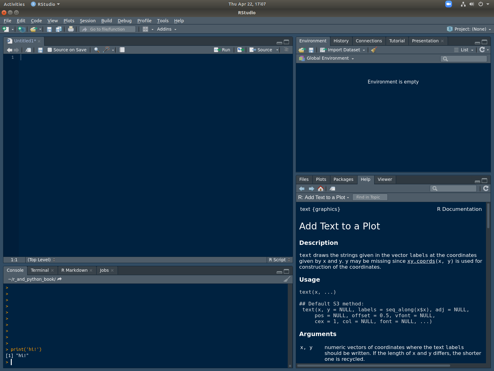
Figure 1.1: RStudio
I changed my “Editor Theme” from the default to “Cobalt” because it’s easier on my eyes. If you are opening RStudio for the first time, you probably see a lot more white. You can play around with the theme, if you wish, after going to Tools -> Global Options -> Appearance.
The console, which is located by default on the lower left panel, is the place that all of your code gets run. For short one-liners, you can type code directly into the console. Try typing the following code in there. Here we are making use of the print() function.
In R, functions are “first-class objects,” which means can refer to the name of a function without asking it to do anything. However, when we do want to use it, we put parentheses after the name. This is called calling the function or invoking the function. If a function call takes any arguments (aka inputs), then the programmer supplies them between the two parentheses. A function may return values to be subsequently used, or it may just produce a “side-effect” such as printing some text, displaying a chart, or read/writing information to an external data source.
During the semester, we will write more complicated code. Complicated code is usually written incrementally and stored in a text file called a script. Click File -> New File -> R Script to create a new script. It should appear at the top left of the RStudio window (see Figure 1.1 ) . After that, copy and paste the following code into your script window.
print('hello world')
print("this program")
print('is not incredibly interesting')
print('but it would be a pain')
print('to type it all directly into the console')
myName <- "Taylor"
print(myName)
This script will run five print statements, and then create a variable called myName. The print statements are of no use to the computer and will not affect how the program runs. They just display messages to the human running the code.
The variable created on the last line is more important because it is used by the computer, and so it can affect how the program runs. The operator <- is the assignment operator. It takes the character constant "Taylor", which is on the right, and stores it under the name myName. If we added lines to this program, we could refer to the variable myName in subsequent calculations.
Save this file wherever you want on your hard drive. Call it awesomeScript.R. Personally, I saved it to my desktop.
After we have a saved script, we can run it by sending all the lines of code over to the console. One way to do that is by clicking the Source button at the top right of the script window (see Figure 1.1 ). Another way is that we can use R’s source() function1. We can run the following code in the console.
# Anything coming after the pound/hash-tag symbol
# is a comment to the human programmer.
# These lines are ignored by R
setwd("/home/taylor/Desktop/")
source("awesomeScript.R")
The first line changes the working directory to Desktop/. The working directory is the first place your program looks for files. You, dear reader, should change this line by replacing Desktop/ to whichever folder you chose to save awesomeScript.R in. If you would like to find out what your working directory is currently set to, you can use getwd().
Every computer has a different folder/directory structure–that is why it is highly recommended you refer to file locations as seldom as possible in your scripts. This makes your code more portable. When you send your file to someone else (e.g. your instructor or your boss), she will have to remove or change every mention of any directory. This is because those directories (probably) won’t exist on her machine.
The second line calls source(). This function finds the script file and executes all the commands found in that file sequentially.
Deleting all saved variables, and then source()ing your script can be a very good debugging strategy. You can remove all saved variables by running rm(list=ls()). Don’t worry–the variables will come back as soon as you source() your entire script again!
1.2 Hello World in Python
First, start by opening Anaconda Navigator. It should look something like this:
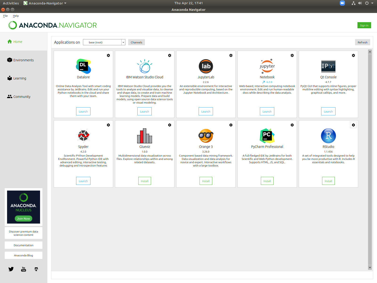
Figure 1.2: Anaconda Navigator
Recall that we will exclusively assume the use of Spyder in this textbook. Open that up now. It should look something like this:
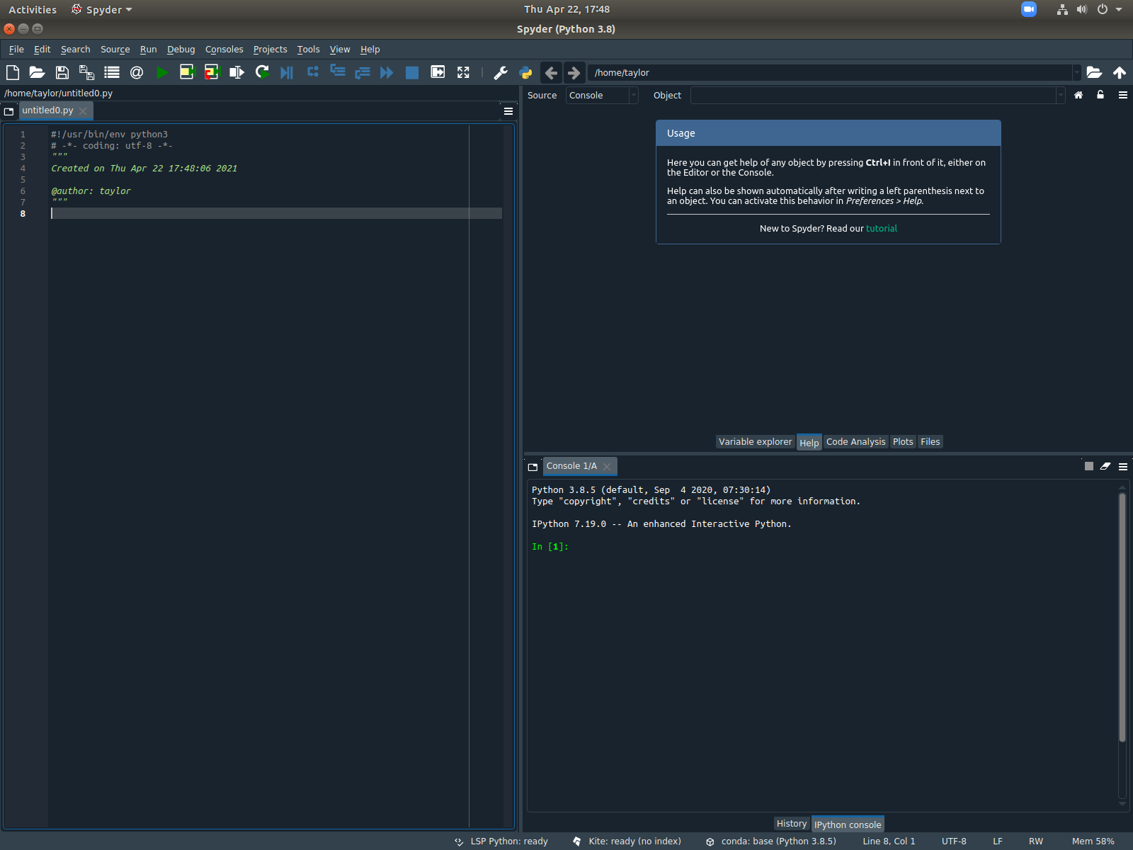
Figure 1.3: Spyder
It looks a lot like RStudio, right? The script window is still on the left hand side, but it takes up the whole height of the window this time. However, you will notice that the console window has moved. It’s over on the bottom right now.
Again, you might notice a lot more white when you open this for the first time. Just like last time, I changed my color scheme. You can change yours by going to Tools -> Preferences and then exploring the options available under the Appearances tab.
Try typing the following line of code into the console.
Already we have many similarities between our two languages. Both R and Python have a print() function, and they both use the same symbol to start a comment: #. Finally, they both define character/string constants with quotation marks In both languages, you can use either single or double quotes.
We will also show below that both languages share the same three ways to run scripts. Nice!
Let’s try writing our first Python script. R scripts end in .r or .R, while Python scripts end in .py. Call this file awesomeScript.py.
# save this as awesomeScript.py
print('hello world')
print("this program")
print('is pretty similar to the last program')
print('it is not incredibly interesting, either')
my_name = "Taylor"
print(my_name)
Notice that the assignment operator is different in Python. It’s an =2.
Just like RStudio, Spyder has a button that runs the entire script from start to finish. It’s the green triangle button (see Figure 1.3 ).
You can also write code to run awesomeScript.py. There are a few ways to do this, but here’s the easiest.
This is also pretty similar to the R code from before. os.chdir() sets our working directory to the Desktop. Then runfile() runs all of the lines in our program, sequentially, from start to finish3.
The first line is new, though. We did not mention anything like this in R, yet. We will talk more about importing modules in section 10.4. Suffice it to say that we imported the os module to make the chdir() function available to us.
1.3 Getting Help
1.3.1 Reading Documentation
Programming is not about memorization. Nobody can memorize, for example, every function and all of its arguments. So what do programmers do when they get stuck? The primary way is to find and read the documentation.
Getting help in R is easy. If you want to know more about a function, type into the console the name of the function with a leading question mark. For example, ?print or ?setwd. You can also use help() and help.search() to find out more about functions (e.g. help(print)). Sometimes you will need to put quotation marks around the name of the function (e.g. ?":").
This will not open a separate web browser window, which is very convenient. If you are using RStudio, you have some extra benefits. Everything will look very pretty, and you can search through the text by typing phrases into the search bar in the “Help” window.
In Python, the question mark comes after the name of the function4 (e.g. print?), and you can use help(print) just as in R.
In Spyder, if you want the documentation to appear in the Help window (it looks prettier), then you can type the name of the function, and then Ctrl-i (Cmd-i on a mac keyboard).
1.3.2 Understanding File Paths
File paths look different on different operating systems. Mac and Linux machines tend to have forward slashes (i.e. /), while Windows machines tend to use backslashes (i.e. \).
Depending on what kind of operating system is running your code, you will need to change the file paths. It is important for everyone writing R and Python code to understand how things work on both types of machines–just because you’re writing code on a Windows machine doesn’t mean that it won’t be run on a Mac, or vice versa.
The directory repeatedly mentioned in the code above was /home/taylor/Desktop. This is a directory on my machine which is running Ubuntu Linux. The leading forward slash is the root directory. Inside that is the directory home/, and inside that is taylor/, and inside that is Desktop/. If you are running MacOS, these file paths will look very similar. The folder home/ will most likely be replaced with Users/.
On Windows, things are a bit different. For one, a full path starts with a drive (e.g. C:). Second, there are backslashes (not forward slashes) to separate directory names (e.g C:\Users\taylor\Desktop).
Unfortunately, backslashes are a special character in both R and Python (read section 3.9 to find out more about this). Whenever you type a \, it will change the meaning of whatever comes after it. In other words, \ is known as an escape character.
In both R and Python, the backslash character is used to start an “escape” sequence. You can see some examples in R by clicking here, and some examples in Python by clicking here. In Python it may also be used to allow long lines of code to take up more than one line in a text file.
The recommended way of handling this is to just use forward slashes instead. For example, if you are running Windows, C:/Users/taylor/Desktop/myScript.R will work in R, and C:/Users/taylor/Desktop/myScript.py will work in Python.
You may also use “raw string constants” (e.g. r'C:\Users\taylor\my_file.txt' ). “Raw” means that \ will be treated as a literal character instead of an escape character. Alternatively, you can “escape” the backslashes by replacing each single backslash with a double backslash. Please read section 3.9 for more details about these choices.
A third way is to tell R to run
awesomeScript.Rfrom the command line, but unfortunately, this will not be discussed in this text. ↩You can use this symbol in R, too, but it is less common.↩
Python, like R, allows you to run scripts from the command line, but this will not be discussed in this text.↩
If you did not install
Anaconda, then this may not work for you because this is an IPython (https://ipython.org) feature.↩