Chapter 3 R vectors versus Numpy arrays and Pandas’ Series
This section is for describing the data types that let us store collections of elements that all share the same type. Data is very commonly stored in this fashion, so this section is quite important. Once we have one of these collection objects in a program, we will be interested in learning how to extract and modify different elements in the collection, as well as how to use the entire collection in an efficient calculation.
3.1 Overview of R
In the previous section, I mentioned that R does not have scalar types–it just has vectors. So, whether you want to store one number (or logical, or character, or …), or many numbers, you will need a vector.
For many, the word “vector” evokes an impression that these objects are designed to be used for performing matrix arithmetic (e.g. inner products, transposes, etc.). You can perform these operations on vectors, but in my opinion, this preconception can be misleading, and I recommend avoiding it. Most of the things you can do with vectors in R have little to do with linear algebra!
How do we create one of these? There are many ways. One common way is to read in elements from an external data set. Another way is to generate vectors from code.
1:10         # consecutive integers
##  [1]  1  2  3  4  5  6  7  8  9 10
seq(1,10,2)  # arbitrary sequences
## [1] 1 3 5 7 9
rep(2,5)     # repeating numbers
## [1] 2 2 2 2 2
# combine elements without relying on a pattern
c("5/2/2021", "5/3/2021", "5/4/2021")
## [1] "5/2/2021" "5/3/2021" "5/4/2021"
# generate Gaussian random variables
rnorm(5)
## [1] -0.98392997  1.70994197  0.77709483 -0.09817682 -0.43579996
c() is short for “combine”. seq() and rep() are short for “sequence” and “replicate”, respectively. rnorm() samples normal (or Gaussian) random variables. There is plenty more to learn about these functions, so I encourage you to take a look at their documentation.
I should mention that functions such as rnorm() don’t create truly random numbers, just pseudorandom ones. Pseudorandom numbers are nearly indecipherable from truly random ones, but the way the computer generates them is actually deterministic.
First, a seed, or starting number is chosen. Then, the pseudorandom number generator (PRNG) maps that number to another number. The sequence of all the numbers appears to be random, but is actually deterministic.
Sometimes you will be interested in setting the seed on your own because it is a cheap way of sharing and communicating data with others. If two people use the same starting seed, and the same PRNG, then they should simulate the same data. This can be important if you want to help other people reproduce the results of code you share. Most of the time, though, I don’t set the seed, and I don’t think about the distinction between random and pseudorandom numbers.
3.2 Overview of Python
If you want to store many elements of the same type (and size) in Python, you will probably need a Numpy array. Numpy is a highly-regarded third party library (Harris et al. 2020) for Python. Its array objects store elements of the same type, just as R’s vectors do.
There are five ways to create numpy arrays (source). Here are some examples that complement the examples from above.
import numpy as np
np.array([1,2,3])
## array([1, 2, 3])
np.arange(1,12,2)
## array([ 1,  3,  5,  7,  9, 11])
np.random.normal(size=3)
## array([-1.49837736,  0.14307108,  0.34530069])
Another option for storing a homogeneous collection of elements in Python is a Series object from the Pandas library. The benefit of these is that they play nicely with Pandas’ data frames (more information about Pandas’ data frames can be found in 8.2), and that they have more flexibility with accessing elements by name ( see here for more information ).
3.3 Vectorization in R
An operation in R is vectorized if it applies to all of the elements of a vector at once. An operator that is not vectorized can only be applied to individual elements. In that case, the programmer would need to write more code to instruct the function to be applied to all of the elements of a vector. You should prefer writing vectorized code because it is usually easier to read. Moreover, many of these vectorized functions are written in compiled code, so they can often be much faster.
Arithmetic (e.g. +, -, *, /, ^, %%, %/%, etc.) and logical (e.g. !, |, &, >, >=, <, <=, ==, etc.) operators are commonly applied to one or two vectors. Arithmetic is usually performed element-by-element. Numeric vectors are converted to logical vectors if they need to be. Be careful of operator precedence if you seek to minimize your use of parentheses.
Note that there are an extraordinary amount of named functions (e.g. sum(), length(), cumsum(), etc.) that operate on entire vectors, as well. Here are some examples.
(1:3) * (1:3)
## [1] 1 4 9
(1:3) == rev(1:3)
## [1] FALSE  TRUE FALSE
sin( (2*pi/3)*(1:4))
## [1]  8.660254e-01 -8.660254e-01 -2.449294e-16  8.660254e-01
In the last example, there is recycling happening. (2*pi/3) is taking three length-one vectors and producing another length-one vector. The resulting length-one vector is multiplied by a length four vector 1:4. The single element in the length one vector gets recycled so that its value is multiplied by every element of 1:4.
This makes sense most of the time, but sometimes recycling can be tricky. Notice that the following code does not produce an error–just a warning: longer object length is not a multiple of shorter object length. Try running it on your machine to confirm this.
3.4 Vectorization in Python
The Python’s Numpy library makes extensive use of vectorization as well. Vectorization in Numpy is accomplished with universal functions, or “ufuncs” for short. Some ufuncs can be invoked using the same syntax as in R (e.g. +). You can also refer to function by its name (e.g. np.sum() instead of +). Mixing and matching is allowed, too.
Ufuncs are called unary if they take in one array, and binary if they take in two. At the moment, there are fewer than \(100\) available, all performing either mathematical operations, boolean-emitting comparisons, or bit-twiddling operations. For an exhaustive list of Numpy’s universal functions, click here. Here are some code examples.
np.arange(1,4)*np.arange(1,4)
## array([1, 4, 9])
np.zeros(5) > np.arange(-3,2)
## array([ True,  True,  True, False, False])
np.exp( -.5 * np.linspace(-3, 3, 10)**2) / np.sqrt( 2 * np.pi)
## array([0.00443185, 0.02622189, 0.09947714, 0.24197072, 0.37738323,
##        0.37738323, 0.24197072, 0.09947714, 0.02622189, 0.00443185])
Instead of calling it “recycling”, Numpy calls reusing elements of a shorter array in a binary operation broadcasting. It’s the same idea as in R, but in general, Python is stricter and disallows more scenarios. For example, try running the following code on your machine. You should receive an error: ValueError: operands could not be broadcast together with shapes (2,) (3,).
If you are working with string arrays, Numpy has a np.char module with many useful functions.
Then there are the Series objects from Pandas. Ufuncs continue to work in the same way on Series objects, and they respect common index values.
s1 = pd.Series(np.repeat(100,3))
s2 = pd.Series(np.repeat(10,3))
s1 + s2
## 0    110
## 1    110
## 2    110
## dtype: int64
If you feel more comfortable, and you want to coerce these Series objects to Numpy arrays before working with them, you can do that. For example, the following works.
s = pd.Series(np.linspace(-1,1,5))
np.exp(s.to_numpy())
## array([0.36787944, 0.60653066, 1.        , 1.64872127, 2.71828183])
In addition, Series objects possess many extra attributes and methods.
ints = pd.Series(np.arange(10))
ints.abs()
## 0    0
## 1    1
## 2    2
## 3    3
## 4    4
## 5    5
## 6    6
## 7    7
## 8    8
## 9    9
## dtype: int64
ints.mean()
## 4.5
ints.floordiv(2)
## 0    0
## 1    0
## 2    1
## 3    1
## 4    2
## 5    2
## 6    3
## 7    3
## 8    4
## 9    4
## dtype: int64
Series objects that have text data are a little bit different. For one, you have to access the .str attribute of the Series before calling any vectorized methods. Here are some examples.
## dtype('O')## 0 False
## 1 False
## 2 False
## 3 True
## dtype: bool## 0 z
## 1 b
## 2 c
## 3 33
## dtype: objectString operations can be a big game changer, and we discuss text processing strategies in more detail in section 3.9.
3.5 Indexing Vectors in R
It is very common to want to extract or modify a subset of elements in a vector. There are a few ways to do this. All of the ways I discuss will involve the square bracket operator (i.e. []). Feel free to retrieve the documentation by typing ?'['.
allElements <- 1:6
allElements[seq(2,6,2)] # extract evens
## [1] 2 4 6
allElements[-seq(2,6,2)] <- 99 # replace all odds with 99
allElements[allElements > 2] # get nums bigger than 2
## [1] 99 99  4 99  6
To access the first element, we use the index 1. To access the second, we use 2, and so on. Also, the - sign tells R to remove elements. Both of these functionalities are very different from Python, as we will see shortly.
We can use names to access elements elements, too, but only if the elements are named.
3.6 Indexing Numpy arrays
Indexing Numpy arrays is very similar to indexing vectors in R. You use the square brackets, and you can do it with logical arrays or index arrays. There are some important differences, though.
For one, indexing is 0-based in Python. The 0th element is the first element of an array. Another key difference is that the - isn’t used to remove elements like it is in R, but rather to count backwards. Third, using one or two : inside square brackets is more flexible in Python. This is syntactic sugar for using the slice() function, which is similar to R’s seq() function.
one_through_ten = np.arange(1, 11)
one_through_ten[np.array([2,3])]
## array([3, 4])
one_through_ten[1:10:2] # evens
## array([ 2,  4,  6,  8, 10])
one_through_ten[::-1] # reversed
## array([10,  9,  8,  7,  6,  5,  4,  3,  2,  1])
one_through_ten[-2] = 99 # second to last
one_through_ten
## array([ 1,  2,  3,  4,  5,  6,  7,  8, 99, 10])
one_through_ten[one_through_ten > 3] # bigger than three
## array([ 4,  5,  6,  7,  8, 99, 10])
3.7 Indexing Pandas’ Series
At a minimum, there is little that is new that you need to learn to go from Numpy arrays to Pandas’ Series objects. They still have the [] operator, and many methods are shared across these two types. The following is almost equivalent to the code above, and the only apparent difference is that the results are printed a little differently.
import pandas as pd
one_through_ten = pd.Series(np.arange(1, 11))
one_through_ten[np.array([2,3])]
## 2    3
## 3    4
## dtype: int64
one_through_ten[1:10:2] # evens
## 1     2
## 3     4
## 5     6
## 7     8
## 9    10
## dtype: int64
one_through_ten[::-1] # reversed
## 9    10
## 8     9
## 7     8
## 6     7
## 5     6
## 4     5
## 3     4
## 2     3
## 1     2
## 0     1
## dtype: int64
one_through_ten[-2] = 99 # second to last
one_through_ten
##  0     1
##  1     2
##  2     3
##  3     4
##  4     5
##  5     6
##  6     7
##  7     8
##  8     9
##  9    10
## -2    99
## dtype: int64
one_through_ten[one_through_ten > 3] # bigger than three
##  3     4
##  4     5
##  5     6
##  6     7
##  7     8
##  8     9
##  9    10
## -2    99
## dtype: int64
one_through_ten.sum()
## 154
However, Pandas’ Series have .loc and .iloc methods. We won’t talk much about these two methods now, but they will become very important when we start to discuss Pandas’ data frames in section 8.2.
3.8 Some Gotchas
3.8.1 Shallow versus Deep Copies
In R, assignment usually produces a deep copy. In the code below, we create b from a. If we modify b, these changes don’t affect a. This takes up more memory, but our program is easier to follow as we don’t have to keep track of connections between objects.
With Numpy arrays in Python, “shallow copies” can be created by simple assignment, or by explicitly constructing a view. In the code below, a, b, c, and d all share the same data. If you modify one, you change all the others. This can make the program more confusing, but on the other hand, it can also improve computational efficiency.
# in python
a = np.array([1,2,3])
b = a # b is an alias
c = a.view() # c is a view
d = a[:]
b[0] = 999
a # two names for the same object in memory
## array([999,   2,   3])
b
## array([999,   2,   3])
c
## array([999,   2,   3])
d
## array([999,   2,   3])
It’s the same story with Pandas’ Series objects. You’re usually making a “shallow” copy.
# in python
import pandas as pd
s1 = pd.Series(np.array([100.0,200.0,300.0]))
s2 = s1
s3 = s1.view()
s4 = s1[:]
s1[0] = 999
s1
## 0    999.0
## 1    200.0
## 2    300.0
## dtype: float64
s2
## 0    999.0
## 1    200.0
## 2    300.0
## dtype: float64
s3
## 0    999.0
## 1    200.0
## 2    300.0
## dtype: float64
s4
## 0    999.0
## 1    200.0
## 2    300.0
## dtype: float64
If you want a “deep copy” in Python, you usually want a function or method called copy(). Use np.copy or np.ndarray.copy when you have a Numpy array.
# in python
a = np.array([1,2,3])
b = np.copy(a)
c = a.copy()
b[0] = 999
a
## array([1, 2, 3])
b
## array([999,   2,   3])
c
## array([1, 2, 3])
Use pandas.Series.copy with Pandas’ Series objects. Make sure not to set the deep argument to False. Otherwise you’ll get a shallow copy.
3.8.2 How R and Python Handle Missing Values
R has NULL, NaN, and NA. Python has None and np.nan. If your eyes are glazing over already and you’re thinking “they all look like the same”–they are not.
R’s NULL and Python’s None are similar. Both represent “nothingness.” This is not the same as 0, or an empty string, or FALSE/False. This is commonly used to detect if a user fails to pass in an argument to a function, or if a function fails to “return” (more information on functions can be found in section 6) anything meaningful.
In R, for example, if a function fails to return anything, then it actually returns a NULL. A NULL object has its own type.
NULL == FALSE
## logical(0)
NULL == NULL
## logical(0)
# create a function that doesn't return anything
# more information on this later
doNothingFunc <- function(a){}
thing <- doNothingFunc() # call our new function
is.null(thing)
## [1] TRUE
typeof(NULL)
## [1] "NULL"
In Python, we have the following.
None == False
## False
None == None
# create a function that doesn't return anything
# more information on this later
## True
def do_nothing_func():
    pass
thing = do_nothing_func()
if thing is None:
    print("thing is None!")
## thing is None!
type(None)
## <class 'NoneType'>
“NaN” stands for “not a number.” NaN is an object of type double in R, and np.nan is of type float in Python. It can come in handy when you (deliberately or accidentally) perform undefined calculations such as \(0/0\) or \(\infty / -\infty\).
# in Python
# 0/0
# the above yields a ZeroDivisionError
import numpy as np
np.inf/np.inf
## nan
np.isnan(np.nan)
## True
“NA” is short for “not available.” Missing data is a fact of life in data science. Observations are often missing in data sets, introduced after joining/merging data sets together (more on this in section 12.3), or arise from calculations involving underflow and overflow. There are many techniques designed to estimate quantities in the presence of missing data. When you code them up, you’ll need to make sure you deal with NAs properly.
# in R
babyData <- c(0,-1,9,NA,21)
NA == TRUE
## [1] NA
is.na(babyData)
## [1] FALSE FALSE FALSE  TRUE FALSE
typeof(NA)
## [1] "logical"
Unfortunately, Python’s support of an NA-like object is more limited. There is no NA object in base Python. And often NaNs will appear in place of an NA. There are a few useful tools, though. The Numpy library offers “masked arrays”, for instance.
Also, as of version 1.0.0, the pandas library has an experimental pd.NA object. However, they warn that “the behaviour of pd.NA can still change without warning.”
import numpy as np
import numpy.ma as ma
baby_data = ma.array([0,-1,9,-9999, 21]) # -9999 "stands for" missing
baby_data[3] = ma.masked
np.average(baby_data)
## 7.25
Be careful of using extreme values to stand in for what should be an NA. Be aware that some data providers will follow this strategy. I recommend that you avoid it yourself. Failing to represent a missing value correctly would lead to extremely wrong calculations!
3.9 An Introduction to Regular Expressions
We have already talked a little about how to work with text data in this book. Regarding Python, section 3.4 mentioned that Pandas Series objects have a .str accessor attribute that has plenty of special methods that will work on string data. The same tools can be used whether or not these Series objects are contained in a Pandas DataFrame.
Regarding R, character vectors were first mentioned in section 3.1. There are many functions that operate on these, too, regardless of whether they are held in a data.frame. The functions might be a little harder to find because they aren’t methods, so pressing <Tab> and using your GUI’s autocomplete feature doesn’t reveal them as easily.
Suppose you’re interested in replacing lowercase letters with uppercase ones, removing certain characters from text, or counting the number of times a certain expression appears. Up until now, as long as you can find a function or method that performs the task, you were doing just fine. If you need to do something with text data, there’s probably a function for it.
Notice what all of these tasks have in common–they all require the ability to find patterns. When your patterns are easy to describe (e.g. find all lowercase “a”s), then all is well. What can make matters more complicated, however, is when the patterns are more difficult to describe (e.g. find all valid email addresses). That is why this section is primarily concerned with discussing regular expressions, which are a tool that help you describe the patterns in text (Wickham and Grolemund 2017) (López 2014).
3.9.1 Literal Characters versus Metacharacters
Every character in a regular expression is interpreted in one of two ways. Either it is interpreted as a
- literal character, or as a
- metacharacter.
If it is a literal character, then the character is the literal pattern. For example, in the regular expression “e”, the character “e” has a literal interpretation. If you seek to capitalize all instances of “e” in the following phrase, you can do it pretty easily. As long as you know which function performs find-and-replace, you’re good. The pattern is trivial to specify.
On the other hand, if I asked you to remove $s from price or salary data, you might have a little more difficulty. This is because $ is a metacharacter in regular expressions, and so it has a special meaning.6 In the examples below, if $ is interpreted as a regular expression, the pattern will not be found at all, despite the prevalence of literal dollar signs.
There are a few functions in R that perform find-and-replace, but in this case, I use gsub(). In Pandas, I can use .str.replace(), to do this. Here are the examples that find patterns that are described by literal characters.
# in R
gsub(pattern = "e", replacement = "E",
     x = "I don't need a regex for this!")
## [1] "I don't nEEd a rEgEx for this!"
# in Python
import pandas as pd
s = pd.Series(["I don't need a regex for this!"])
s.str.replace(pat="e",repl="E")
## 0 I don't nEEd a rEgEx for this!
## dtype: objectOn the other hand, here are a few examples that remove dollar signs. We generally have two options to recognize symbols that happen to be metacharacters.
- We can escape the dollar sign. That means you need to put a backslash (i.e.
\) before the dollar sign. The backslash is a metacharacter looks at the character coming after it, and it either removes the special meaning from a metacharacter, or adds special meaning to a literal character. - Alternatively, we can tell the function to ignore regular expressions.
gsub()can takefixed=TRUE, and.str.replace()can takeregex=False.
3.9.2 The Trouble With Backslashes: Escape Sequences
You might have noticed above and gotten confused–sometimes in Python and in R, we need two backslashes instead of one. This is because backslashes have another purpose that can complicate our using them to escape metacharacters. They also help us write untypeable characters, also known as escape sequences. We need to be able to do this even if we aren’t using regular expressions.
For instance, consider the way we type the “newline” character. Even though it is understood by the computer as one character, it takes us two keystrokes to write it with our keyboard. \ is one character, and n is another, but together they are one!
strs in Python and character vectors in R will look for these combinations by default. When we specify regular expressions with strings, the backslashes will be used first for this purpose. Their regular expression purpose is a second priority.
The reason we used \\$ in the above example is to escape the second backslash. \$ is not a special character, but Python and R will handle it differently. Python will not recognize it, and it won’t complain that it didn’t. On the other hand, R will throw an error that it can’t recognize it.
nchar('\$') # R gets confused
## Error: '\$' is an unrecognized escape in character string starting "'\$"
There is another way to deal with this issue–raw strings! Raw strings make life easier because they do not interpret backslashes as the beginning of escape sequences. You can make them in R and Python by putting an “r” in front of the quotation marks. However, it is slightly more complicated in R because you need a delimiter pair inside the quotation marks–for more information type ?Quotes in your R console.
3.9.3 More Examples of Using Regular Expressions
Regular expressions that match many different types of characters are often very useful–these are called character classes. For example, . represents any character except a newline, \d represents any digit, and \s represents any whitespace character. You can sometimes capitalize the letters in the regular expression to get the opposite pattern.
# anonymize phone numbers in R
gsub(pattern = r"{\d}", replacement = "X", x = "(202)555-0191")
## [1] "(XXX)XXX-XXXX"
# remove everything that isn't a number in Python
pd.Series(["$100"]).str.replace(pat="\D",repl="")
## 0 100
## dtype: objectMany character classes feature an opening and closing square brackets. For instance, [1-5] matches any digit between \(1\) and \(5\) (inclusive), [aeiouy] matches any lowercase vowel, and [\^\-] matches either ^ or - (we had to escape these two metacharacters because we are only interested in the literal pattern).
# remove vowels in R
gsub(pattern = "[aeiouy]", replacement = "",
     x = "Can you still read this?")
## [1] "Cn  stll rd ths?"
Concatenating two patterns, one after another, forms a more specific pattern to be matched.
# convert date formats in Python
s = pd.Series(["2021-10-23","2021:10:23"])
s.str.replace(pat="[:\-]",repl="/")
## 0    2021/10/23
## 1    2021/10/23
## dtype: object
If you would like one pattern or another to appear, you can use the alternation operator |.
# one or the other in Python
pd.Series(["this","that"]).str.contains(pat="this|that")
## 0    True
## 1    True
## dtype: bool
In addition to concatenation, alternation, and grouping, there are more general ways to quantify how many times the desired pattern will appear. ? means zero or one time, * means zero or more, + will mean one or more, and there are a variety of ways to be even more specific with curly braces (e.g. {3,17} means anywhere from three to seventeen times).
# detect double o's in R
grepl(pattern = "o{2}", x = c("look","book","box", "hellooo"))
## [1]  TRUE  TRUE FALSE  TRUE
# detects phone number formats in Python
s = pd.Series(["(202)555-0191","202-555-0191"])
s.str.contains(pat=r"\(\d{3}\)\d{3}-\d{4}")
## 0 True
## 1 False
## dtype: boolNotice in the double “o” example, the word with three matched. To describe that not being desirable requires the ability to look ahead of the match, to the next character, and evaluate that. You can look ahead, or behind, and make assertions about what patterns are required or disallowed.
| Lookaround Regex | Meaning |
|---|---|
(?=pattern) |
Positive looking ahead for pattern |
(?!pattern) |
Negative looking ahead for pattern |
(?<=pattern) |
Positive looking behind for pattern |
(?<!pattern) |
Negative looking behind for pattern |
After oo we specify (?!o) to disallow a third, trailing o.
# exactly two "o"s in Python?
s = pd.Series(["look","book","box", "hellooo"])
s.str.contains(pat="oo(?!o)")
## 0     True
## 1     True
## 2    False
## 3     True
## dtype: bool
However, this does not successfully remove "hellooo" because it will match on the last two “o”s of the word. To prevent this, we can prepend a (?<!o), which disallows a leading “o”, as well. In R, we also have to specify perl=TRUE to use Perl-compatible regular expressions.
# exactly two "o"s in R
grep(pattern = "(?<!o)oo(?!o)",
     x = c("look","book","box", "hellooo"), perl = TRUE)
## [1] 1 2
We also mention anchoring. If you only want to find a pattern at the beginning of text, use ^. If you only want to find a pattern at the end of text, use $. Below we use .str.extract(), whose documentation makes reference to capture groups. Capture groups are just regular expressions grouped inside parentheses (e.g. (this)).
3.10 Exercises
3.10.1 R Questions
Let’s flip some coins! Generate a thousand flips of a fair coin. Use rbinom, and let heads be coded as 1 and tails coded as 0.
- Assign the thousand raw coin flips to a variable
flips. Make sure the elements are integers, and make sure you flip a “fair” coin (\(p=.5\)). - Create a length
1000logicalvectorcalledisHeads. Whenever you get a heads, make sure the corresponding element isTRUEandFALSEotherwise. - Create a variable called
numHeadsby tallying up the number of heads. - Calculate the percent of time that the number changes in
flips. Assign your number toacceptanceRate. Try to write only one line of code to do this.
Compute the elements of the tenth order Taylor approximation to \(\exp(3)\) and store them in taylorElems. Do not sum them. Use only one expression, and do not use any loop. The approximation is,
\[
1 + 3 + 3^2/2! + 3^3/3! + \cdots 3^{10}/10!
\]
You want to store each of those eleven numbers separately in a numeric vector.
Do the following.
- Create a vector called
numsthat contains all consecutive integers from \(-100\) to \(100\). - Create a
logicalvectorthat has the same length as the above, and containsTRUEwhenever an element of the above is even, andFALSEotherwise. Call itmyLogicals. - Assign the total number of
TRUEs tototalEven. - Create a
vectorcalledevensof all even numbers from the abovevector. - Create a
vectorcalledreversethat holds the reversed elements ofnums.
Let’s say we wanted to calculate the following sum \(\sum_{i=1}^N x_i\). If \(N\) is large, or most of the \(x_i\)s are large, then we might bump up against the largest allowable number. This is the problem of overflow. The biggest integer and biggest floating point can be recovered by typing .Machine$integer.max and .Machine$double.xmax, respectively.
- Assign
sumThesetoexp(rep(1000,10)). Are they finite? Can you sum them? If everything is all good, assignTRUEtoallGood. - Theoretically, is the logarithm of the sum less than
.Machine$double.xmax? AssignTRUEorFALSEtonoOverflowIssue. - Assign the naive log-sum of these to
naiveLogSum. Is the naive log sum finite? - Compute
betterSum, one that doesn’t overflow, using the log-sum-exp trick:
\[
\log\left( \sum_{i=1}^{10} x_i \right) = \log\left( \sum_{i=1}^{10} \exp[ \log(x_i) - m] \right) + m
\]
\(m\) is usually chosen to be \(\max_i \log x_i\). This is the same formula as above, which is nice. You can use the same code to combat both overflow and underflow.
e) If you’re writing code, and you have a bunch of very large numbers, is it better to store those numbers, or store the logarithm of those numbers? Assign your answer to whichBetter. Use either the phrase "logs" or "nologs".
Say you have a vector of prices of some financial asset:
Use the natural logarithm and convert this vector into a vector of log returns. Call the variable
logReturns. If \(p_t\) is the price at time \(t\), the log return ending at time \(t\) is \[\begin{equation} r_t = \log \left( \frac{p_t}{p_{t-1}} \right) = \log p_t - \log p_{t-1} \end{equation}\]Do the same for arithmetic returns. These are regular percent changes if you scale by \(100\). Call the variable
arithReturns. The mathematical formula you need is \[\begin{equation} a_t = \left( \frac{p_t - p_{t-1} }{p_{t-1}} \right) \times 100 \end{equation}\]
Consider the mixture density \(f(y) = \int f(y \mid x) f(x) dx\) where
\[\begin{equation} Y \mid X = x \sim \text{Normal}(0, x^2) \end{equation}\] and
\[\begin{equation} X \sim \text{half-Cauchy}(0, 1). \end{equation}\] This distribution is a special case of a prior distribution that is used in Bayesian statistics (Carvalho, Polson, and Scott 2009). Note that the second parameter of the Normal distribution is its variance, not its standard deviation.
Suppose further that you are interested in calculating the probability that one of these random variables ends up being too far from the median:
\[\begin{equation} \mathbb{P}[|Y| > 1] = \int_{y : |y| > 1} f(y)dy = \int_{y : |y| > 1} \int_{-\infty}^\infty f(y \mid x) f(x) dx dy. \end{equation}\]
The following steps will demonstrate how you can use the Monte-Carlo (Robert and Casella 2005) method to approximate this probability.
Simulate \(X_1, \ldots, X_{5000}\) from a \(\text{half-Cauchy}(0, 1)\) and call these samples
xSamps. Hint: you can simulate from a \(t\) distribution with one degree of freedom to sample from a Cauchy. Once you have regular Cauchy samples, take the absolute value of each one.Simulate \(Y_1 \mid X_1, \ldots, Y_{5000} \mid X_{5000}\) and call the samples
ySamps.Calculate the approximate probability using
ySampsand call itapproxProbDev1.Why is simply “ignoring”
xSamps(i.e. not using it in the averaging part of the computation), the samples you condition on, “equivalent” to “integrating out \(x\)”? Store a string response as a length \(1\) character vector calledintegratingOutResp.Calculate another Rao-Blackwellized Monte Carlo estimate of \(\mathbb{P}[|Y| > 1]\) from
xSamps. Call itapproxProbDev2. Hint: \(\mathbb{P}[|Y| > 1] = \mathbb{E}[\mathbb{P}(|Y| > 1 \mid X) ]\). Calculate \(\mathbb{P}(|Y| > 1 \mid X=x)\) with pencil and paper, notice it is a function in \(x\), apply that function to each ofxSamps, and average all of it together.Are you able to calculate an exact solution to \(\mathbb{P}[|Y| > 1]\)?
Store the ordered uppercase letters of the alphabet in a length \(26\) character vector called myUpcaseLetters. Do not hardcode this. Use a function, along with the variable letters.
Create a new vector called
withReplacementsthat’s the same as the previousvector, but replace all vowels with"---". Again, do not hardcode this. Find a function that searches for patterns and performs a replacement whenever that pattern is found.Create a length \(26\) logical vector that is
TRUEwhenever an element oflettersis a consonant, andFALSEeverywhere else. Call itconsonant.
3.10.2 Python Questions
Let’s flip some coins (again)! Generate a thousand flips of a fair coin. Use np.random.binomial, and let heads be coded as 1 and tails coded as 0.
- Assign the thousand raw coin flips to a variable
flips. Make sure the elements are integers, and make sure you flip a “fair” coin (\(p=.5\)). - Create a length
1000listofbools calledis_heads. Whenever you get a heads, make sure the corresponding element isTrueandFalseotherwise. - Create a variable called
num_headsby tallying up the number of heads. - Calculate the percent of time that the number changes in
flips. Assign your number toacceptance_rate. Try to write only one line of code to do this.
Create a Numpy array containing the numbers \(1/2, 1/4, 1/8, \ldots, 1/1024\) Make sure to call it my_array.
Do the following:
- Create a
np.arraycallednumsthat contains one hundred equally-spaced numbers starting from \(-100\) and going to \(100\) (inclusive). - Create a
boolnp.arraythat has the same length as the above, and containsTRUEwhenever an element of the above is less than ten units away from \(0\), andFALSEotherwise. Call itmy_logicals. - Assign the total number of
Trues tototal_close. - Create a
np.arraycalledevensof all even numbers from the abovenp.array(even numbers are necessarily integers). - Create a
np.arraycalledreversethat holds the reversed elements ofnums.
Let’s say we wanted to calculate the following sum \(\sum_{i=1}^N x_i\). We run into problems when this sum is close to \(0\), too. This is the problem of underflow. The smallest positive floating point can be recovered by typing np.nextafter(np.float64(0),np.float64(1)).
- Assign
sum_theseto the length ten array \((e^{-1000}, \ldots, e^{-1000})\). Usenp.exp(np.repeat(-1000,10)). Are the elements nonzero? Can you sum them? Is the sum correct? If everything is all good, assignTruetoall_good. - Theoretically, for which range of positive numbers is the logarithm of the number farther from \(0\) than the number itself? Assign the lower bound to
lower_bound, and the upper bound toupper_bound. Hint:lower_boundis \(0\) because we’re only looking at positive numbers, and because the logarithm is \(-\infty\). - Assign the naive log-sum of
sum_thesetonaive_log_sum. Is the naive log sum finite on your computer? Should it be? - Compute
better_sum, one that doesn’t underflow, using the log-sum-exp trick. This one should be bounded away from \(-\infty\).
\[
\log\left( \sum_{i=1}^{10} x_i \right) = \log\left( \sum_{i=1}^{10} \exp[ \log(x_i) - m] \right) + m =
\]
\(m\) is usually chosen to be \(\max_i \log x_i\)
e) If you’re writing code, and you have a bunch of very small positive numbers (e.g. probabilities, densities, etc.), is it better to store those small numbers, or store the logarithm of those numbers? Assign your answer to which_better. Use either the phrase "logs" or "nologs".
Use pd.read_csv to correctly read in "2013-10_Citi_Bike_trip_data_20K.csv" as a data frame called my_df. Make sure to read autograding_tips.html.
- Extract the
"starttime"column into a separateSeriescalleds_times. - Extract date strings of those elements into a
Seriescalleddate_strings. - Extract time strings of those elements into a
Seriescalledtime_strings.
We will make use of the Monte Carlo method below. It is a technique to approximate expectations and probabilities. If \(n\) is a large number, and \(X_1, \ldots, X_n\) is a random sample drawn from the distribution of interest, then \[\begin{equation} \mathbb{P}(X > 6) \approx \frac{1}{n}\sum_{i=1}^n \mathbf{1}(X_i > 6). \end{equation}\] If you haven’t seen an indicator function before, it is defined as
\[\begin{equation} \mathbf{1}(X_i > 6) = \begin{cases} 1 & X_i > 6 \\ 0 & X_i \le 6 \end{cases}. \end{equation}\]
If you wanted to visualize it, \(\mathbf{1}(x > 6)\) looks like this.
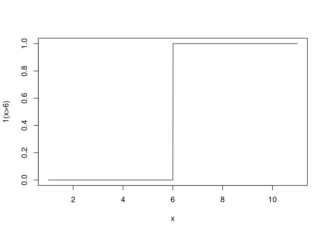
Figure 3.1: An Indicator Function
So, the sum in this expression is just a count of the number of elements that are greater than \(6\).
Evaluate exactly the probability that a normal random variable with mean \(5\) and standard deviation \(6\) is greater than \(6\). Assign it to the variable
exact_exceedance_probin Python.Simulate \(1e3\) times from a standard normal distribution (mean 0 and variance 1). Call the samples
stand_norm_samps.Calculate a Monte Carlo estimate of \(\mathbb{P}(X > 6)\) from these samples. Call it
approx_exceedance_prob1.Simulate \(1e3\) times from a normal distribution with mean \(5\) and standard deviation \(6\). Call the samples
norm_samps. Don’t use the old samples in any way.Calculate a Monte Carlo estimate of \(\mathbb{P}(X > 6)\) from these new
norm_samps. Call itapprox_exceedance_prob2.
Alternatively, we can approximate expectations using the same technique as above. If \(\mathbb{E}[g(X)]\) exists, \(n\) is a large number, and \(W_1, \ldots, W_n\) is a random sample drawn from the distribution of interest, then
\[\begin{equation} \mathbb{E}[g(W)] \approx \frac{1}{n}\sum_{i=1}^n g(W_i). \end{equation}\]
Here’s a new distribution. It is a mixture distribution, specifically a finite mixture of normal distributions: \(f(y) = f(y \mid X=1)P(X=1) + f(y \mid X=0)P(X=0)\) where
\[\begin{equation} Y \mid X=0 \sim \text{Normal}(0, 2) \\ Y \mid X=1 \sim \text{Normal}(10, 2) \end{equation}\] and
\[\begin{equation} X \sim \text{Bernoulli}(.5). \end{equation}\]
Both \(f(y \mid X=0)\) and \(f(y \mid X=1)\) are bell-curved, and \(f(y)\) looks like this
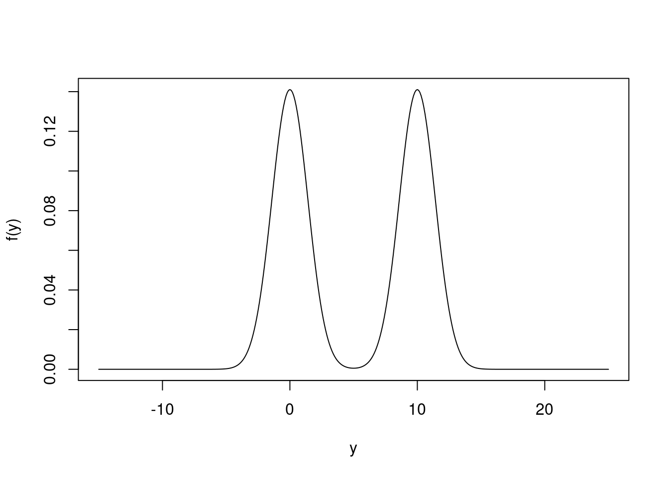
Figure 3.2: The Marginal Density of Y
Evaluate exactly \(\mathbb{E}[Y] = \mathbb{E}[ \mathbb{E}(Y \mid X) ]\). Assign it to the variable
exact_meanin Python.Simulate \(1e3\) times from the Bernoulli distribution. Call the samples
bernoulli_flipsSimulate \(Y_1 \mid X_1, \ldots, Y_{1000} \mid X_{1000}\) and call the samples
cond_norm_samps.Calculate a Monte Carlo estimate of \(\mathbb{E}[Y]\) from
cond_norm_samps. Call itapprox_ave_1. Why is simply “ignoring”bernoulli_flips, the samples you condition on, “equivalent” to “integrating them out?”Calculate a Rao-Blackwellized Monte Carlo estimate of \(\mathbb{E}[Y]\) from
bernoulli_flips. Call itapprox_ave_2. Hint: \(\mathbb{E}[Y] = \mathbb{E}[\mathbb{E}(Y \mid X) ]\). Calculate \(\mathbb{E}(Y \mid X_i)\) exactly, and evaluate that function on each \(X_i\) sample, and then average them together. Rao-Blackwellization is a variance-reduction technique that allows you come up with lower-variance estimates given a fixed computational budget.
References
Carvalho, Carlos M., Nicholas G. Polson, and James G. Scott. 2009. “Handling Sparsity via the Horseshoe.” In Proceedings of the Twelth International Conference on Artificial Intelligence and Statistics, edited by David van Dyk and Max Welling, 5:73–80. Proceedings of Machine Learning Research. Hilton Clearwater Beach Resort, Clearwater Beach, Florida USA: PMLR. https://proceedings.mlr.press/v5/carvalho09a.html.
Harris, Charles R., K. Jarrod Millman, Stéfan J. van der Walt, Ralf Gommers, Pauli Virtanen, David Cournapeau, Eric Wieser, et al. 2020. “Array Programming with NumPy.” Nature 585 (7825): 357–62. https://doi.org/10.1038/s41586-020-2649-2.
López, Félix. 2014. Mastering Python Regular Expressions : Leverage Regular Expressions in Python Even for the Most Complex Features. Birmingham, UK: Packt Pub.
Robert, Christian P., and George Casella. 2005. Monte Carlo Statistical Methods (Springer Texts in Statistics). Berlin, Heidelberg: Springer-Verlag.
Wickham, Hadley, and Garrett Grolemund. 2017. R for Data Science: Import, Tidy, Transform, Visualize, and Model Data. 1st ed. O’Reilly Media, Inc.
The dollar sign is useful if you only want to find certain patterns that finish a line. It takes the characters preceding it, and says, only look for that pattern if it comes at the end of a string.↩